6 Calculus of functions of two variables
Finally, having developed some preliminary algebra, we turn to perhaps the main topic of the module: generalising calculus to functions of two variables. If you can master this generalisation, you will be able to understand how calculus should work for functions of any number of variables – we restrict to the case of two variables since the notation is easy, and we can visualise the ideas best. But there are no new ideas involved when considering functions of more variables.
6.1 Functions \(\mathbb{R}^2\longrightarrow\mathbb{R}\)
6.1.1 3-dimensional visualisation
Just as a function \(f:\mathbb{R}\longrightarrow\mathbb{R}\) is a function with input in \(\mathbb{R}\) and output in \(\mathbb{R}\), a function \(f:\mathbb{R}^2\longrightarrow\mathbb{R}\) is a function with input in \(\mathbb{R}^2\) and output in \(\mathbb{R}\). So the input to the function is a pair \((x,y)\), and the output is a single real number \(z=f(x,y)\). For example, the function \(f(x,y)=x^2+y^2\) takes two inputs, \(x\) and \(y\), and returns an output \(x^2+y^2\), so that \(f(2,1)=2^2+1^2=5\), for example.
Here are some examples of functions of \(2\) variables:
\(z=x+y\);
\(z=e^{xy}\);
\(z=\sin x^2/\cos(e^y)\)
Just as \(y=f(x)\) is not the only way to specify a 2-dimensional picture, and some shapes are only specified with a more general relationship \(f(x,y)=0\) (e.g., a circle is given by \(x^2+y^2=r^2\)), we may want to consider more general relationships than those given by \(z=f(x,y)\), and may consider more general loci \(f(x,y,z)=0\).
We can visualise loci like this with 3-dimensional graphs, where the \(x,y\)-plane is regarded as horizontal, and the \(z\)-direction gives a vertical direction.
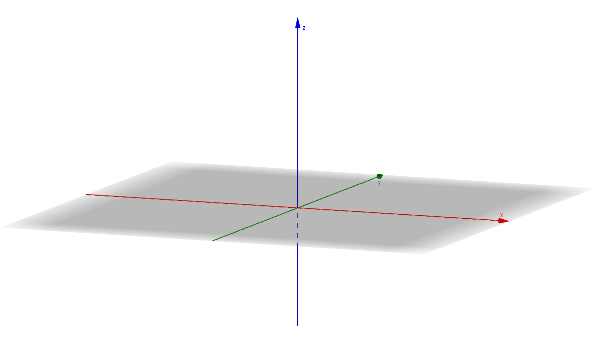
Figure 6.1: Three-dimensional Cartesian coordinates
Using this visualisation, we can give equations for some well-known geometrical shapes:
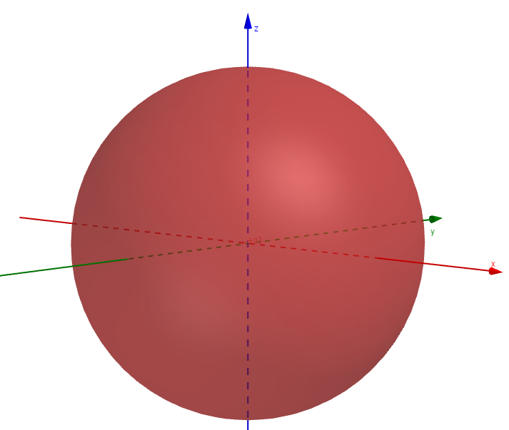
Figure 6.2: The sphere

Figure 6.3: The cylinder

Figure 6.4: The (double) cone
We can also rotate any curve around an axis; to rotate a locus \(f(x,y)=0\) around the \(z\)-axis, we replace the equation with \(f(r,z)=0\), where \(z\) is the vertical axis, and where \(r=\sqrt{x^2+y^2}\). In fact, the last two examples are instances of this. As a further example, we recall the paraboloid, whose equation is given by \(z=x^2+y^2\).
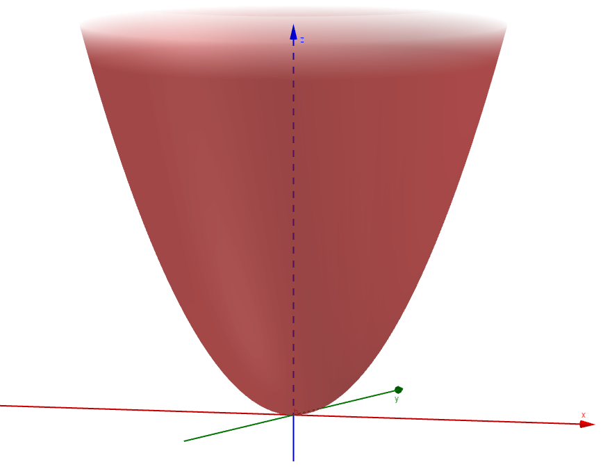
Figure 6.5: The paraboloid
6.1.2 Level Curves
It is harder to visualise 3 dimensions on the page than 2 dimensions. But we are familiar with ways of doing this – maps with contours are common in geography, for example. We can do the same thing here.
For each number \(c\), the equation \(f(x,y)=c\) is the equation of a curve in the plane. This is called the level curve of \(f\) at \(c\). By drawing various level curves, we can often get a good description of the function \(f\). One can think of this like a contour map where \(c\) is the altitude of a point on the graph.

Figure 6.6: Level curves
Drawn in the \((x,y)\)-plane, the level curves are circles:

Figure 6.7: Circular level curves for the cone
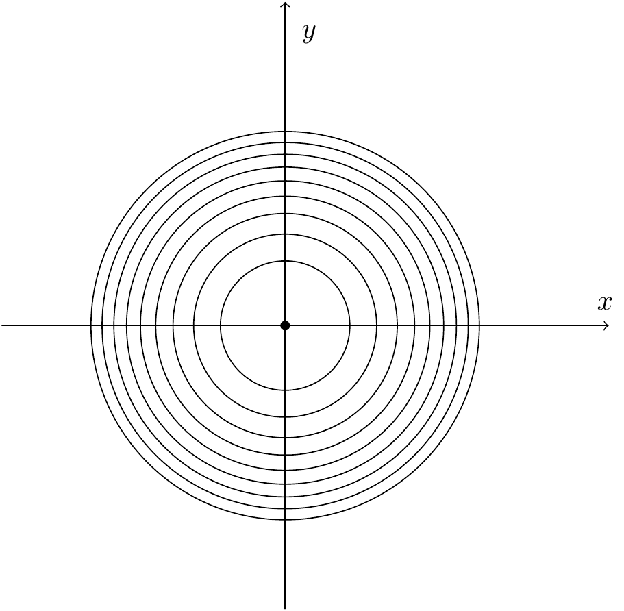
Figure 6.8: Circular level curves for the paraboloid
Example 6.6 Suppose the height above sea level of a mountain in metres is given by \(f(x,y) =3000-2x^2 - 3y^4\). Draw a contour map of this surface.
We can see that the highest point is \(f(0,0)=3000\). As \(x\) and \(y\) increase, the altitude decreases. The level curves (contours) look like this:

Figure 6.9: Level curves for the example
Example 6.7 Sketch some level curves for the function \(f(x,y)=y-x^2\).
We fix a constant \(c\). The level curve of \(f\) at \(c\) is given by \(y-x^2=c\); that is, \(y=x^2+c\). This is a parabola in the \((x,y)\) plane passing through the point \((0,c)\). The level curves for \(c = 0,1,...,4\) look as follows: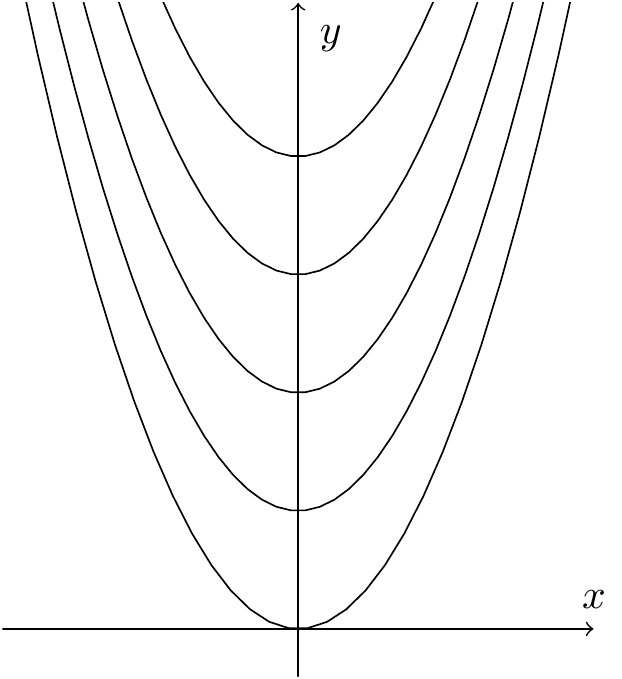
Figure 6.10: Level curves for the example
6.2 Partial Derivatives
6.2.1 Review of the 1-dimensional case
Remember that we can find the maximum or minimum of a function by looking at its turning points. For many functions, we can differentiate to find these turning points; differentiation gives us the gradient of a function, and the turning points occur where the gradient is \(0\). So we can find the turning points where the derivative (another word for differential) is \(0\).
We can tell whether functions are maxima or minima by looking at the second derivative. The second derivative is the derivative of the first derivative. If the second derivative is positive, the first derivative is increasing, so the gradient is increasing, and this happens when the turning point is a minimum, and the gradient moves from negative (going down to the minimum) to positive (going up from the minimum). Similarly, if the second derivative is negative, the first derivative is decreasing, and this corresponds to a maximum. (If the second derivative is \(0\), this can be either a maximum, or a minimum, or a point of inflection.)
The second derivative can be identified from the Taylor series expansion of a function \(f\) – recall that the Taylor series of the function \(f(x)\) around \(x=a\) is given by \[f(x)=f(a)+(x-a)f'(a)+\frac{(x-a)^2}{2!}f''(a)+\cdots.\] Alternatively, if we write \(x=a+h\), we get: \[f(a+h)=f(a)+hf'(a)+\frac{h^2}{2!}f''(a)+\cdots.\]
We will explain that for functions of two variables, there is a similar notion of a Taylor expansion. Once again, the tangent (now a plane, rather than a line) is given by the degree \(1\) terms in the Taylor expansion; stationary points will be those points where these degree \(1\) terms vanish. Further (although this will require more work), we can determine the nature of the stationary points by looking at the degree 2 terms in the Taylor series. For this reason, we will also need to study quadratic curves as well as lines, and we will do this in the next chapter, before returning to calculus to classify stationary points for functions of two variables.
6.2.2 Partial differentiation
Suppose \(f\) is a function of two variables, \(x\) and \(y\). For example, we may have \[f(x,y)=3x^2-3y^2+8xy.\]
As usual we can imagine this as plotted in 3 dimensions, two for the variables \(x\) and \(y\), and one for the value of the function, plotted on the \(z\)-axis.
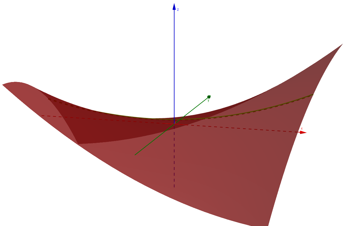
Figure 6.11: A function of two variables
One way to visualise \(f\) is to regard \(y\) as some fixed value \(b\), and to let \(x\) vary. Then we can differentiate \(f\) with respect to \(x\), which gives the gradient of \(f\) in the slice \(y=b\) at the point \(x\). So we think of the slice \(y=b\), which has equation \(z=f(x,b)=3x^2-3b^2+8xb\), where \(b\) is a constant. Then we can differentiate purely using the \(x\)-variable. The usual notation for this is \[\frac{\partial f}{\partial x}=6x+8b.\] (Sometimes, especially to save space, we use the notation \(f_x\) to denote this expression.) So the gradient at \((x,b)\) is \(6x+8b\), and so at \(x=a\), the gradient is \(6a+8b\).
Notice the notation here; when we have more than one variable, and
differentiate with respect to just one of them, we call this partial
differentiation, and write \(\frac{\partial f}{\partial x}\) instead of
\(\frac{df}{dx}\). (If you are doing MAS115, you might like to know that
this funny \(\partial\) is written \partial in LaTeX.)
Let’s reflect on what this gradient measures. We are essentially looking at a cross-section of the graph, going through the slice \(y=b\). Every slice contains a 2-dimensional picture, plotting \(f\) (or \(z\)) against the single variable \(x\).
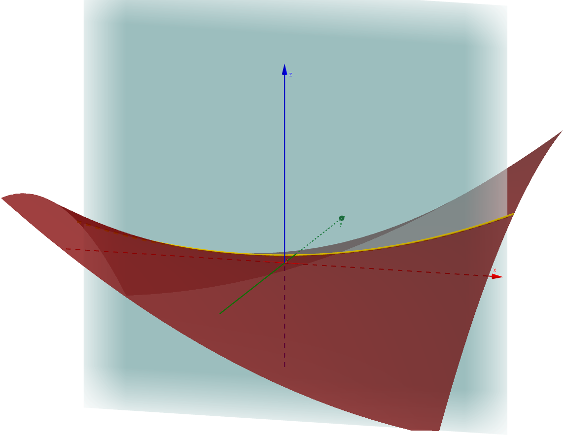
Figure 6.12: A cross-section slice of the surface
The picture here shows the original graph intersected with a slice \(y=b\) (in fact, \(y=0.1\) here).
The differential is measuring the amount \(f\) changes when \(x\) changes; if \(x\) changes from \(a\) to \(a+h\), say, then \(f\) should change by approximately \((6a+8b)h\). It is important to stress that only \(x\) is changing here, and \(y\) is fixed. So we are moving from \((a,b)\) to \((a+h,b)\), and then \(f(a,b)\) should change to \(f(a+h,b)\), which is approximately \(f(a,b)+(6a+8b)h\). (This is essentially just the first couple of terms of the Taylor series; we would get a more accurate approximation by using more terms.)
This sort of differentiation says nothing about what happens when \(y\) varies.
For this, we could fix \(x\) to be some value \(a\), and let \(y\) vary. Then we can differentiate \(f\) with respect to \(y\), and get the gradient of \(f\) in the slice \(x=a\) at \(y\).
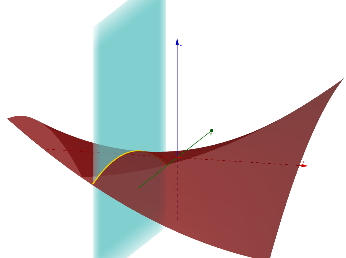
Figure 6.13: The other cross-section slice of the surface
image
The picture here shows the slice of the original graph corresponding to \(x=a\) (\(x=-0.15\) here).
We get \(-6y+8a\); what this means is that if we move from \((a,b)\) moves to \((a,b+k)\), then \(f(a,b+k)\) is approximately \(f(a,b)+(-6b+8a)k\).
Here, we see nothing about what happens when \(x\) varies.
The notation for this is \[\frac{\partial f}{\partial y}=-6y+8x,\] or sometimes \(f_y\).
Here’s a formal definition:Definition 6.1 The partial derivative of a function \(f(x,y)\) with respect to \(x\), denoted \(\frac{\partial f}{\partial x}\) (or sometimes \(f_x\)), is defined by
\[\frac{\partial f}{\partial x}=\lim_{\delta x\to0}\frac{f(x+\delta x,y)-f(x,y)}{\delta x}.\]
So the partial derivative \(\frac{\partial f}{\partial x}\) is the derivative of \(f\) with respect to \(x\), holding \(y\) constant.
Likewise, the partial derivative of \(f(x,y)\) with respect to \(y\), denoted \(\frac{\partial f}{\partial y}\) is defined by
\[\frac{\partial f}{\partial y}=\lim_{\delta y\to0}\frac{f(x,y+\delta y)-f(x,y)}{\delta y},\]
the derivative of \(f\) with respect to \(y\), holding \(x\) constant.
Example 6.8 For \(f(x,y)=x^2+y^2\), the paraboloid above, we see that the partial derivative with respect to \(x\) is \(\frac{\partial f}{\partial x}=2x\), and the partial derivative with respect to \(y\) is \(\frac{\partial f}{\partial y}=2y\). We get the partial derivative with respect to \(x\) by differentiating with respect to \(x\) as usual and treating \(y\) as a constant. (Similarly for the partial derivative with respect to \(y\).)
At the point on the surface with coordinates \((1,-\tfrac{1}{2},\tfrac{5}{4})\), \(\frac{\partial f}{\partial x}=2\) and \(\frac{\partial f}{\partial y}=-1\).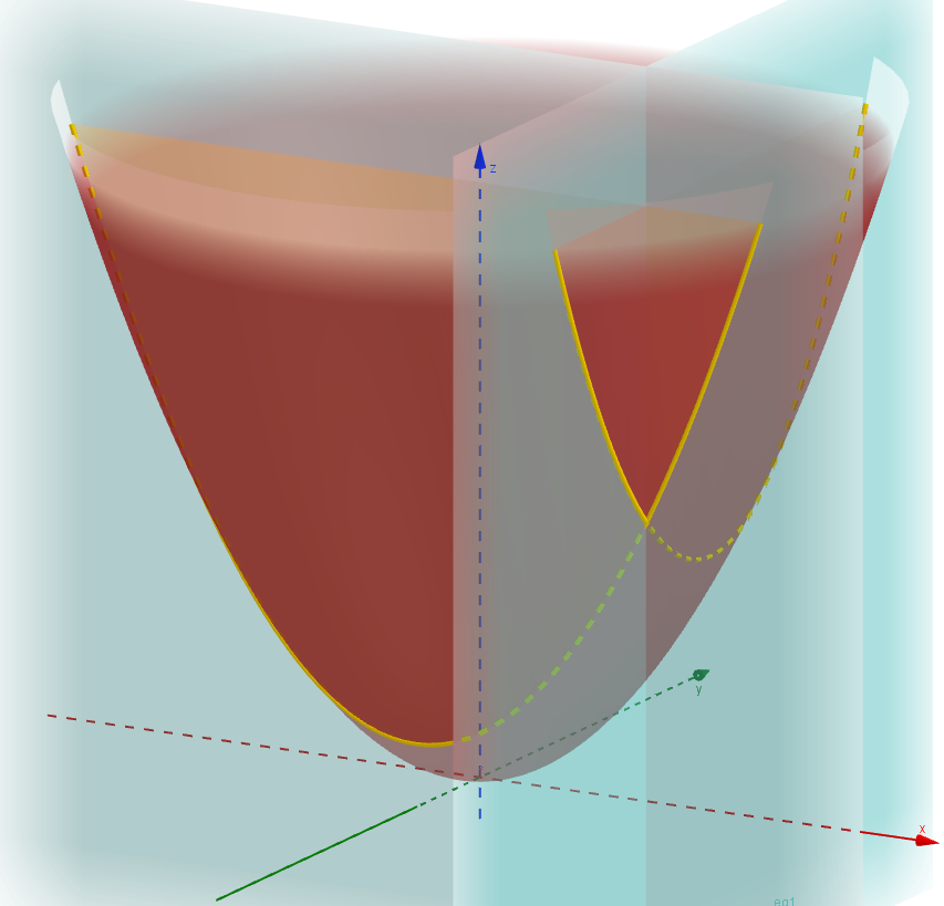
Figure 6.14: Slices through the paraboloid
Example 6.9 If \(f(x,y)=ax+by+c\), \[f_x=\frac{\partial f}{\partial x}=a,\qquad f_y=\frac{\partial f}{\partial y}=b.\]
Example 6.10 If \(f(x,y)=x^3+x^2y+4x^2y^3\), \[f_x=\frac{\partial f}{\partial x}=3x^2+2xy+8xy^3,\qquad f_y=\frac{\partial f}{\partial y}=x^2+12x^2y^2.\]
6.2.3 Approximations for small increments
Recall that if \(f(x)\) is a function of one variable and \(h=\delta x\) is a small change in the \(x\) direction, \[\frac{\delta f}{\delta x}\approx\frac{df}{dx}.\] Here \(\frac{\delta f}{\delta x}\) is the slope of the chord joining the points \((x,f(x))\) and \((x+\delta x,f(x+\delta x))\) and \(\frac{df}{dx}\) is the slope of the tangent line at the point \((x,f(x))\) to the curve given by the graph of \(f\).
So, we have \[\delta f\approx\frac{df}{dx}\delta x.\] Now let’s go back to considering functions of two variables. For \(y\) fixed and small \(\delta x\), \[\frac{\delta f}{\delta x}\approx\frac{\partial f}{\partial x}\qquad\text{i.e.,}\qquad\delta f\approx\frac{\partial f}{\partial x}\delta x.\] For \(x\) fixed and small \(\delta y\): \[\frac{\delta f}{\delta y}\approx\frac{\partial f}{\partial y}\qquad\text{i.e.,}\qquad\delta f\approx\frac{\partial f}{\partial y}\delta y.\] Allowing both \(x\) and \(y\) to vary, with small \(\delta x\) and \(\delta y\),
\[\delta f\approx\frac{\partial f}{\partial x}\delta x+\frac{\partial f}{\partial y}\delta y.\]
Example 6.11 The power \(P=P(E,R)\) consumed in an electrical resistor is given by \(P=E^2/R\). Here \(E\) is the voltage through the resistor (in volts), \(R\) is the resistance (in ohms) and \(P\) the power in watts. Suppose \(E=200\)V and \(R=8\Omega\). Then \(P=5000\)W. Estimate the change in \(P\) if \(E\) is increased by \(5\)V and \(R\) is decreased by \(0.2\Omega\).
At \((E,R)=(200,8)\), \[\begin{aligned} \frac{\partial P}{\partial E}&=\frac{2E}{R}=\frac{2(200)}{8}=50,\\ \frac{\partial P}{\partial R}&=-\frac{E^2}{R^2}=-\frac{200^2}{8^2}=-625.\end{aligned}\] So, \[\begin{aligned} \delta P&\approx\frac{\partial P}{\partial E}\delta E+\frac{\partial P}{\partial R}\delta R\\ &= 50\delta E-625\delta R=50(5)+(-625)(-0.2)=250+125=375.\end{aligned}\] Thus we estimate the change in \(P\) to be 375W.Example 6.12 Again \(P=E^2/R\). Estimate the percentage change in \(P\) if \(E\) is increased by \(0.2\%\) and \(R\) is decreased by \(0.3\%\).
Since \(\delta E=\frac{2}{1000}E\) and \(\delta R=-\frac{3}{1000}R\), we have \(\frac{\delta E}{E}=\frac{2}{1000}\) and \(\frac{\delta R}{R}=-\frac{3}{1000}\).
As before, \(\delta P\approx\frac{\partial P}{\partial E}\delta E+\frac{\partial P}{\partial R}\delta R\). So \[\begin{aligned} \frac{\delta P}{P}&=\frac{\delta P}{E^2/R}\approx 2\frac{\delta E}{E}-\frac{\delta R}{R}\\ &=2\frac{2}{1000}-\frac{-3}{1000}=\frac{7}{1000}.\end{aligned}\] Thus \(P\) increases by approximately \(0.7\%\).6.2.4 The Taylor series up to degree 1
So far, we’ve mostly thought about how \(f\) changes when we move from \((a,b)\) to a nearby point by moving parallel to an axis. But we could instead consider the more general situation where we move from \((a,b)\) in an arbitrary direction. That is, we could move in a particular direction, and see how the function changes. This gives the notion of a directional derivative. We won’t give a formal definition here (leaving it to MAS211), but we are interested in beginning to develop the Taylor series for a function in two variables. So we would like to move from \((a,b)\) to \((a+h,b+k)\), and see how the function’s value changes; this is exactly what the differentiation process computes.
As above, we can simply combine the two changes above, by starting at \((a,b)\) and moving parallel to the \(x\)-axis to \((a+h,b)\), and then parallel to the \(y\)-axis, to \((a+h,b+k)\). Then we have worked out how \(f\) changes: \[f(a+h,b+k)\approx f(a,b)+\frac{\partial f}{\partial x}h+\frac{\partial f}{\partial y}k.\] This follows from writing \(\delta x\) for the change in \(x\) and \(\delta y\) for the change in \(y\) (so \(\delta x=h\) and \(\delta y=k\)), and then the result that the change in \(f\) is approximately \[\delta f\approx \frac{\partial f}{\partial x}\delta x+\frac{\partial f}{\partial y}\delta y.\]
For example, if \(f(x,y)=x^3y^2\), we get \[\frac{\partial f}{\partial x}=3x^2y^2,\qquad\frac{\partial f}{\partial y}=2x^3y\] At \((x,y)=(a,b)\), we have \[\frac{\partial f}{\partial x}=3a^2b^2,\qquad\frac{\partial f}{\partial y}=2a^3b\] and so \[f(a+h,b+k)\approx f(a,b)+3a^2b^2h+2a^3bk.\]
You can see that this resembles the first couple of terms of the Taylor series for functions of \(1\) variable mentioned above. We can view this as the first degree part of a 2-dimensional Taylor series for \(f\) about \((a,b)\). In order to go further, we will need some higher partial derivatives.
6.2.5 A warning example
We will give some results in the module that hold for “nice” functions. Every function you are likely to meet in practice is almost certain to be “nice”. But there are functions which are not nice. The area of analysis considers what “nice” means in various contexts, and we can try to understand functions which are not nice. This section (not to be lectured) will show you why it’s important to be careful! It’s always important to check the hypotheses of any result you want to apply.
Here is a function which is not nice, in that it does not satisfy the properties one expects to see in functions that might arise in applications. We’ll see further results later on which are generally true, in that it’s not unreasonable to quote the results without thinking, but for which there are actually counterexamples. There is a very interesting short book, “Counterexamples in Analysis” by Gelbaum and Olmsted, where you can find many more strange examples!
I strongly recommend that you look at these functions in Geogebra, using the 3D Graphics View.
We start with a function \(f(x,y)\) such that, for all \(x=a\), we can draw the function \(f(a,y)\) as a continuous function of the variable \(y\), and for all \(y=b\), we can draw \(f(x,b)\) as a continuous function of the variable \(x\). Informally, this means that we can draw a graph of the function which takes \(y\in\mathbb{R}\) to \(f(a,y)\in\mathbb{R}\) without taking our pen off the paper, and similarly for the function that takes \(x\in\mathbb{R}\) to \(f(x,b)\in\mathbb{R}\). However, as a function of two variables, it is not continuous.
Consider the function \[f(x)=\left\{ \begin{array}{ll} \frac{xy}{x^2+y^2},&\mbox{for $(x,y)\ne(0,0)$},\\ 0,&\mbox{for $(x,y)=(0,0)$}. \end{array} \right.\]
For any fixed slice \(y=b\ne0\), we have \[f(x,b)=\frac{bx}{b^2+x^2},\] and this function can be drawn nicely without taking the pen off the paper, which is (informally!) a reasonable definition of continuous.
For the slice \(y=0\), we have \(f(x,0)=0\) for all \(x\), so this is certainly continuous.
The function is symmetric in \(x\) and \(y\), so we can get the same results for slices \(x=a\ne0\) and \(x=0\).
So any slice through this graph has a continuous cross-section.
But what if we take a slice at another angle? Let’s look at the slice \(x=y\). Whenever \(x=y\), we have \[f(x,x)=\frac{x\times x}{x^2+x^2}=\frac{1}{2},\] except for \(x=0\), where \(f(0,0)=0\). So the function is discontinuous at \((0,0)\) as there are points arbitrarily close to \((0,0)\) where the function takes values of \(\frac{1}{2}\). (Similarly, \(f(x,-x)=-\frac{1}{2}\).)
There are discontinuous functions which are not only continuous in any slice \(x=a\) or \(y=b\), but in every slice where \(y=mx\) for any \(m\). We adapt the previous example: \[f(x)=\left\{ \begin{array}{ll} \frac{x^2y}{x^4+y^2},&\mbox{for $(x,y)\ne(0,0)$},\\ 0,&\mbox{for $(x,y)=(0,0)$}. \end{array} \right.\] Again, use Geogebra to see what the function looks like. As \[f(x,mx)=\frac{x^2\times mx}{x^4+m^2x^2}=\frac{mx}{x^2+m^2},\] we see that \(f(x,mx)\to0\) as \(x\to0\), and the function is continuous in the slice \(y=mx\).
However, although the function tends to \(0\) in any slice through the origin, there are nevertheless points arbitrarily close to \((0,0)\) where the value is \(\frac{1}{2}\): \[f(a,a^2)=\frac{a^2\times a^2}{a^4+(a^2)^2}=\frac{1}{2}.\]
6.3 More about partial derivatives
6.3.1 The Chain Rule
Let \(f(x,y)\) be a function of two variables. Suppose that \(x\) and \(y\) depend in turn on \(t\). So as \(t\) varies, then \(x\) and \(y\) both vary, leading to a change in \(f\). What is \(\frac{df}{dt}\)? We know from above that \[\delta f\approx\frac{\partial f}{\partial x}\delta x+\frac{\partial f}{\partial y}\delta y.\] We can divide both sides by \(\delta t\), and take limits as \(\delta t\to0\).
This gives the Chain Rule:
For \(f\) a function of two variables \(x\) and \(y\), which are themselves functions of \(t\), \[\frac{df}{dt}=\frac{\partial f}{\partial x}\cdot\frac{dx}{dt}+\frac{\partial f}{\partial y}\cdot\frac{dy}{dt}.\]
Example 6.13 Let \(f(x,y)=x^2+y^2\), with \(x=t^2\) and \(y=3t\). Calculate \(\frac{df}{dt}\).
\[\frac{\partial f}{\partial x}=2x,\qquad\frac{\partial f}{\partial y}=2y,\qquad\frac{dx}{dt}=2t,\qquad\frac{dy}{dt}=3.\] So \[\begin{aligned} \frac{df}{dt}&=\frac{\partial f}{\partial x}\cdot\frac{dx}{dt}+\frac{\partial f}{\partial y}\cdot\frac{dy}{dt}\\ &=(2x)(2t)+(2y)(3)=(2t^2)(2t)+(6t)(3)=4t^3+18t.\end{aligned}\] Alternatively, \[f(t)=f(x(t),y(t))=(t^2)^2+(3t)^2=t^4+9t^2.\] Hence, \[\frac{df}{dt}=4t^3+18t.\]Example 6.14 An isosceles triangle has two equal sides of length \(r\)cm, enclosing an angle \(\theta\). At time \(t=0\), \(r=2\) and \(\theta=\frac{\pi}{3}\). But \(r\) is growing at a rate of \(2\)cm per second and \(\theta\) is growing at a rate of \(2\) degrees per second. At what rate is the area of the triangle growing?
Let \(A\) be the area. We want \(\frac{dA}{dt}\). By the Chain Rule, \[\frac{dA}{dt}=\frac{\partial A}{\partial r}\cdot\frac{dr}{dt}+\frac{\partial A}{\partial \theta}\cdot\frac{d\theta}{dt}.\] We have \(A=\frac{1}{2}r^2\sin\theta\). So \[\begin{aligned} \frac{\partial A}{\partial r}=r\sin\theta,\qquad&\frac{\partial A}{\partial\theta}=\frac{1}{2}r^2\cos \theta,\\ \frac{dr}{dt}=2\text{cm}/\text{s},\qquad&\frac{d\theta}{dt}=\frac{\pi}{90}\text{rad}/\text{s}.\end{aligned}\] Thus \[\begin{aligned} \frac{dA}{dt}&=2r\sin\theta+\frac{\pi}{180}r^2\cos\theta\\ &=2\cdot\frac{\sqrt{3}}{2}\cdot2+\frac{\pi}{180}\cdot4\cdot\frac{1}{2}\\ &=2\sqrt{3}+\frac{\pi}{90}\text{cm}^2/\text{s}\approx3.499\text{cm}^2/\text{s}.\end{aligned}\]
As a variant, suppose \(f\) is a function of \(2\) variables \(x\), \(y\), and also suppose that \(x=x(s,t)\), \(y=y(s,t)\) are functions of 2 variables. This case will be important when we do changes of variable for integration of functions of two variables.
Then: \[\frac{\partial f}{\partial s}=\frac{\partial f}{\partial x}\cdot\frac{\partial x}{\partial s}+\frac{\partial f}{\partial y}\cdot\frac{\partial y}{\partial s}\] (we simply regard \(t\) as a constant), and similarly for \(\frac{\partial f}{\partial t}\).
6.3.2 Jacobians and integration by substitution
We already began to motivate the generalisation of integration by substitution; let’s now fill in some more details.
For functions of two variables, integration will represent the volume under a surface \(z=f(x,y)\). We approximate the volume by summing the volumes of the cuboids of base widths \(\delta x\times\delta y\) and height \(f(x,y)\). We want to apply a change of variable \(x=x(u,v)\), \(y=y(u,v)\), and consider the integral of \(f(u,v)\). The base of the cuboid is a rectangle of size \(\delta u\,\delta v\). We know from above that \[\begin{aligned} \delta x&\approx\frac{\partial x}{\partial u}\delta u+\frac{\partial x}{\partial v}\delta v\\ \delta y&\approx\frac{\partial y}{\partial u}\delta u+\frac{\partial y}{\partial v}\delta v,\end{aligned}\] i.e., \[\begin{pmatrix}\delta x\\\delta y\end{pmatrix}=\begin{pmatrix}\frac{\partial x}{\partial u}&\frac{\partial x}{\partial v}\\\frac{\partial y}{\partial u}&\frac{\partial y}{\partial v}\end{pmatrix}\begin{pmatrix}\delta u\\\delta v\end{pmatrix}.\] We also know that when we act by a matrix, areas get scaled by the determinant of the matrix. So it is this determinant which plays the same role of the scaling factor in the two-variable integral as the differential \(\frac{dx}{du}\) plays in the one-variable case.
Definition 6.2 Let \(x=x(u,v)\), \(y=y(u,v)\). The Jacobian \(\frac{\partial(x,y)}{\partial(u,v)}\) is defined to be
\[\frac{\partial(x,y)}{\partial(u,v)}= \begin{vmatrix} \frac{\partial x}{\partial u}&\frac{\partial x}{\partial v}\\ \frac{\partial y}{\partial u}&\frac{\partial y}{\partial v} \end{vmatrix}=\det\begin{pmatrix} \frac{\partial x}{\partial u}&\frac{\partial x}{\partial v}\\ \frac{\partial y}{\partial u}&\frac{\partial y}{\partial v} \end{pmatrix}.\]
Example 6.15 Let \(x=r\cos\theta\), \(y=r\sin\theta\). Then \[\begin{aligned} \frac{\partial(x,y)}{\partial(r,\theta)}&= \begin{vmatrix} \frac{\partial x}{\partial r}&\frac{\partial x}{\partial \theta}\\ \frac{\partial y}{\partial r}&\frac{\partial y}{\partial \theta} \end{vmatrix}=\begin{vmatrix} \cos\theta&-r\sin\theta\\ \sin\theta&r\cos\theta \end{vmatrix}\\ &=r\cos^2\theta+r\sin^2\theta=r(\cos^2+\sin^2)=r.\end{aligned}\] So when we convert integrals in \(x\) and \(y\) to use polar coordinates \(r\) and \(\theta\), we need to use the formula:
\[dx\,dy=r\,dr\,d\theta.\]
We’ll see many more examples in the chapters on integration.
For now, we’ll quickly look at properties of the Jacobian.
For functions of one variable, we know that \(\frac{dy}{dx}=\frac{1}{\frac{dx}{dy}}\).
The analogous statement for functions of two variables doesn’t work:
Example 6.16 Let \(x=r\cos\theta\), \(y=\sin\theta\). So then \(r=\sqrt{x^2+y^2}\) and \(\theta=\tan^{-1}(\frac{y}{x})\) (in the right half plane).
We have \(\frac{\partial x}{\partial r}=\cos \theta\), but \[\frac{\partial r}{\partial x}=\frac{2x}{2\sqrt{x^2+y^2}}=\frac{x}{r}=\cos\theta\ne\frac{1}{\frac{\partial x}{\partial r}}.\]
So things work a bit differently in the two variable case. However, when we use Jacobians, we do get the same result.
Theorem 6.1 Let \(x=x(u,v)\), \(y=y(u,v)\) and also \(u=u(s,t)\), \(v=v(s,t)\). Then, \[\frac{\partial(x,y)}{\partial(s,t)}=\frac{\partial(x,y)}{\partial(u,v)}\cdot\frac{\partial(u,v)}{\partial(s,t)}.\]
Actually, it’s much easier conceptually than this proof makes it look! The left-hand side measures how much larger a small rectangle becomes when we transform the variables from \(s\) and \(t\) to \(x\) and \(y\); the right-hand side measures how much larger a small rectangle becomes when we first transform the varaibles from \(s\) and \(t\) to \(u\) and \(v\), and then from \(u\) and \(v\) to \(x\) and \(y\). Clearly these ought to measure the same thing.
Corollary 6.1 In the situation of the preceeding theorem, \[\frac{\partial(x,y)}{\partial(u,v)}=1\left/\frac{\partial(u,v)}{\partial(x,y)}\right..\]
Proof. We take \((s,t)=(x,y)\) in the theorem; then the left-hand side becomes \[\frac{\partial(x,y)}{\partial(x,y)}=\begin{vmatrix} \frac{\partial x}{\partial x}&\frac{\partial x}{\partial y}\\ \frac{\partial y}{\partial x}&\frac{\partial y}{\partial y} \end{vmatrix}=\begin{vmatrix}1&0\\0&1\end{vmatrix}=1,\] so the theorem becomes \[1=\frac{\partial(x,y)}{\partial(u,v)}\cdot\frac{\partial(u,v)}{\partial(x,y)}.\]
6.3.3 Directional derivatives and the gradient
Let’s consider again a function \(z=f(x,y)\), and a point \((x_0,y_0,z_0)\) on the surface. We’ve seen how to work out \(\frac{\partial f}{\partial x}\) and \(\frac{\partial f}{\partial y}\) at any point. These compute how \(f\) changes in the \(x\)- and \(y\)-directions. We can look at changes in any direction!
Let’s pick a vector \((a,b)\) of length \(1\). Then we can just look how the function changes with small changes in the direction of \((a,b)\). So let \(h\) be a small number, and we can look at \[f(x_0+ha,y_0+hb)-f(x_0,y_0),\] and we get a natural notion of directional derivative: \[(\nabla_{(a,b)}f)(x_0,y_0)=\lim_{h\to0}\frac{f(x_0+ha,y_0+hb)-f(x_0,y_0)}{h}\] (if this limit exists), just like for usual differentiation for functions of \(1\)-variable.
(As an aside, this symbol \(\nabla\) has several names, but a common one
is “nabla”, and indeed the LaTeX symbol is got with \nabla, for those
of you doing MAS115.)
The Taylor series suggests that (as long as \(f\) is suitably differentiable): \[f(x_0+ha,y_0+hb)-f(x_0,y_0)\approx ha\frac{\partial f}{\partial x}+hb\frac{\partial f}{\partial y},\] which means that \[\begin{aligned} (\nabla_{(a,b)}f)(x_0,y_0)&=a\frac{\partial f}{\partial x}+b\frac{\partial f}{\partial y}\\ &=\left(\frac{\partial f}{\partial x},\frac{\partial f}{\partial y}\right).(a.b),\end{aligned}\] where this is the (2-dimensional) dot product, which is, in turn, simply the matrix product \[\left(\frac{\partial f}{\partial x}~~\frac{\partial f}{\partial y}\right)\begin{pmatrix}a\\b\end{pmatrix}.\]
So these directional derivatives are essentially easily got from the vector \(\left(\frac{\partial f}{\partial x},\frac{\partial f}{\partial y}\right)\) of partial derivatives. This vector is often known as the gradient of \(f\), and is denoted \(\nabla f\). So \[\nabla_{(a,b)}f=\nabla f.(a,b).\]
Let’s ask ourselves what this gradient vector really measures. We’ve understood the directional derivative at \((x_0,y_0)\) in the direction \((a,b)\) as the gradient in the graph \(z=f(x,y)\) as we move a small distance in the direction of some unit vector \((a,b)\) from \((x_0,y_0)\). So this gradient somehow measures the steepness of \(z=f(x,y)\) in the direction \((a,b)\) at \((x_0,y_0)\). But we know how to write the dot product of two vectors in terms of the two vectors: we have \[\begin{aligned} |\nabla_{(a,b)}f|&=|\nabla f.(a,b)|\\ &=|\nabla f|.|(a,b)|\cos\theta\\ &=|\nabla f|\cos\theta,\end{aligned}\] if \(\nabla f\) and \((a,b)\) have an angle of \(\theta\) between them, as \((a,b)\) is a unit vector. So we see that the choice of \((a,b)\) which maximises the directional derivative is the choice where \(\cos\theta\) is as large as possible, i.e., where \(\theta=0\). But this means that \((a,b)\) and \(\nabla f\) are in the same direction! And, further, the slope in this direction is given by \(|\nabla f|\), so the size of \(\nabla f\) tells us how steep the function is. So we have shown that:
Given a point on a surface \(z=f(x,y)\), the direction in which the gradient is steepest is given by \(\nabla f=\left(\frac{\partial f}{\partial x},\frac{\partial f}{\partial y}\right)\), and the size of the gradient in this direction is \(|\nabla f|\).
Again, all these results will hold true for functions of more variables, but it is so often useful to restrict attention to 2 variables, since it allows us to visualise the results better.
Example 6.17 If \(z=f(x,y)=\cos x\cos y+x^2-y\), then \(\nabla f=(-\sin x\cos y+2x,-\cos y\sin y-1)\), and the directional derivative at \((0,0,1)\) in the direction of \((\tfrac{1}{\sqrt{2}},\tfrac{1}{\sqrt{2}})\) is \[(0,-1).(\frac{1}{\sqrt{2}},\frac{1}{\sqrt{2}})=-\frac{1}{\sqrt{2}}.\]
Finally, let’s note that we could reformulate the first order terms in the Taylor series. We have seen that \[f(x_0+h,y_0+k)=f(x_0,y_0)+hf_x(x_0,y_0)+kf_y(x_0,y_0)+\cdots.\] But now we can notice that we could write \[f(x_0+h,y_0+k)=f(x_0,y_0)+(h,k).\nabla f(x_0,y_0)+\cdots.\] We won’t use the \(\nabla\) notation in the rest of the module, but you will probably see it in future modules.
6.3.4 The tangent plane and normal vectors
Just as for the case of curves, we can take tangents to a surface at a point. Indeed, the tangent to a curve can be regarded as the best straight line which approximates the curve at a point; the tangent to a surface can be regarded as the best plane which approximates the curve at a point.
As indicated above, if \(h\) is a small change in the \(x\) direction, and \(y\) is a small change in the \(y\) direction, then \[f(a+h,b+k)\approx f(a,b)+h\frac{\partial f}{\partial x}(a,b)+k\frac{\partial f}{\partial y}.\] So if you ‘sit’ on the graph of \(z=f(x,y)\) at \((x_0,y_0,z_0)\) and look to a nearby point \((x,y,z)\), you get the following small changes: \[\delta x=h=x-x_0,\qquad\delta y=k=y-y_0,\qquad\delta z=z-z_0,\] and these are combined to give: \[z-z_0=f(x_0+\delta x,y_0+\delta y)-f(x_0,y_0)\approx\frac{\partial f}{\partial x}(x_0,y_0)(x-x_0)+\frac{\partial f}{\partial y}(x_0,y_0)(y-y_0).\]
Definition 6.3 The tangent plane to the surface \(z = f(x,y)\) at \((x_0,y_0,z_0)\) is: \[z-z_0=\frac{\partial f}{\partial x}(x_0,y_0)(x-x_0)+\frac{\partial f}{\partial y}(x_0,y_0)(y-y_0).\]
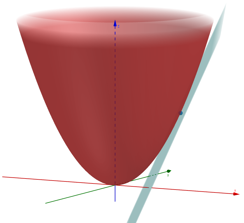
Figure 6.15: The tangent plane to the paraboloid at (2,1,5)
The tangent plane to a surface at a point:
passes through the point;
slopes in the same directions at the point as the surface does.
We’ll define stationary points a little later – just as for curves, the stationary points for surfaces will be the points where the tangent plane is flat.
We have already remarked that given an equation \(ax+by+cz=0\), we can view this as the set of all \((x~y~z)\) which are perpendicular to \((a~b~c)\), since we could rewrite the equation as the dot product of \((a~b~c)\) and \((x~y~z)\). So \(ax+by+cz=0\) is a plane; it is perpendicular to \((a~b~c)\), and passes through the origin. As before, \(ax+by+cz=d\) simply translates the plane in a parallel direction; it remains orthogonal to \((a~b~c)\).
We can combine this and the previous section to give the notion of the normal to a function of two variables at a point, by taking the normal to the tangent plane at the point.
Example 6.20 Find the tangent plane and normal vector to \(z=x^2+y^2\) at \((1,2,5)\).
We first find the tangent plane by computing the first partial derivatives: \(\frac{\partial z}{\partial x}=2x\) and \(\frac{\partial z}{\partial y}=2y\). At the given point, \(\frac{\partial z}{\partial x}=2\) and \(\frac{\partial z}{\partial y}=4\). Then the tangent plane is \[z-5=2(x-1)+4(y-2),\] or \(2x+4y-z=5\).
The normal to this plane is therefore in the direction \((2,4,-1)\). Further, it passes through \((1,2,5)\), so the normal is given in parametric form as \((1,2,5)+(2,4,-1)t=(1+2t,2+4t,5-t)\).As in the \(1\)-variable case, a stationary point is one which is approximately “flat” at the point, meaning that the function doesn’t change when you compare \((a,b)\) with \((a+h,b+k)\), at least up to the first order terms. From the Taylor series, this means \[\frac{\partial f}{\partial x}=\frac{\partial f}{\partial y}=0.\] Equivalently, the tangent plane at \((a,b)\) should be flat.
We’d like to discuss the nature of the stationary points. In the same way as the \(1\)-variable case, functions can have a maximum:
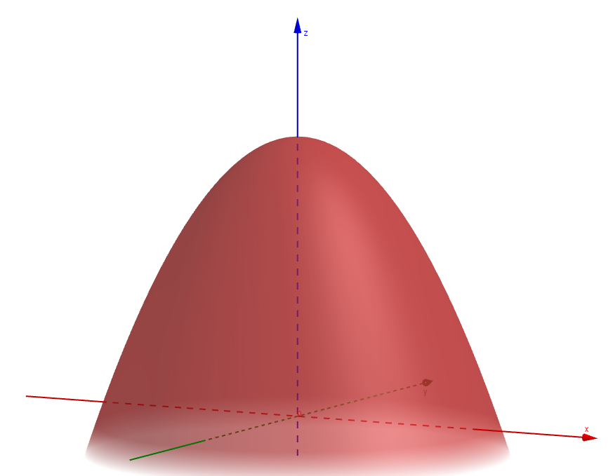
Figure 6.16: A maximum
where the function looks like a hill.
Similarly, functions can have a minimum:
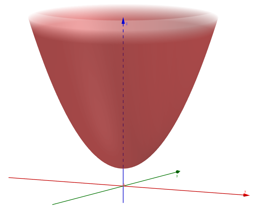
Figure 6.17: A minimum
where the function looks like a bowl.
Later we will discuss how to decide whether a stationary point is a maximum, a minimum, or something else. Indeed, something new can happen here – it is quite possible for a stationary point to be neither a maximum nor a minimum. Indeed, we can have a saddle point:

Figure 6.18: A saddle point
There are some slices through this picture which look as if the given point is a minimum, and others which look as if the given point is a maximum. We will consider this in more detail later.
Let’s merely note from the pictures that the level curves for maxima and minima look like ellipses, while the level curves at saddle points look like hyperbolas; we’ll discuss these curves in the next chapter.
6.4 Higher partial derivatives
6.4.1 Definition
As for standard differentiation, we can repeat the operation, and get higher partial derivatives, denoted \(\frac{\partial^2 f}{\partial x^2}\) (that is, the partial derivative with respect to \(x\) of \(\frac{\partial f}{\partial x}\)) and \(\frac{\partial^2 f}{\partial y^2}\) (the partial derivative with respect to \(y\) of \(\frac{\partial f}{\partial y}\)).
There’s a new feature – we can first take the partial derivative with respect to \(x\) and then with respect to \(y\), or vice versa:
Example 6.21 Let \(f(x,y) = x^2y^2\). Then \[\begin{aligned} \frac{\partial f}{\partial x}&=2xy^2,&\frac{\partial^2f}{\partial y\,\partial x}&=\frac{\partial}{\partial y}\left(\frac{\partial f}{\partial x}\right)=4xy,\\ \frac{\partial f}{\partial y}&=2x^2y,&\frac{\partial^2 f}{\partial x\,\partial y}&=\frac{\partial}{\partial x}\left(\frac{\partial f}{\partial y}\right)=4xy.\end{aligned}\]
Notice that in these examples we get the same answer for the mixed second-order partial derivatives, independent of the order. It turns out that for any nice function you are likely to encounter in practice, this gives the same answer as first taking the partial derivative with respect to \(y\), and then with respect to \(x\). In symbols, \[\frac{\partial^2f}{\partial y\,\partial x}=\frac{\partial^2f}{\partial x\,\partial y}.\]
Proof. Let \[G=f(x+\delta x,y+\delta y)+f(x,y)-f(x+\delta x,y)-f(x,y+\delta y).\] Firstly, we have: \[\begin{aligned} G&=[f(x+\delta x,y+\delta y)-f(x+\delta x,y)]-[f(x,y+\delta y)-f(x,y)]\\ &\approx f_y(x+\delta x,y)\delta y-f_y(x,y)\delta y\\ &=\delta y[f_y(x+\delta x,y)-f_y(x,y)]\\ &\approx\delta y\,\delta x\, f_{yx}(x,y).\end{aligned}\]
Similarly, \(G\approx\delta x\,\delta y\, f_{xy}(x,y)\). So \(f_{yx}=f_{xy}\).6.4.1.1 More warning examples
No function that we encounter in this module – aside from the next example! – and probably no function that you will meet in any module, will have the property that its mixed partial derivatives are different. But they do exist, and it’s important to realise that there is a hypothesis in the theorem above – when the hypothesis is not valid, the conclusion isn’t valid either! Here is an example (not lectured) where things go wrong. This is a slight refinement of the example in section 6.2.5.
But first, we’ll warm up with a simpler warning example, along similar lines, where a pair of limits does not commute:Example 6.24 Plot the function below with Geogebra, and try to use the visualisation to verify the assertions that follow: \[f(x)=\left\{ \begin{array}{ll} \frac{x^2-y^2}{x^2+y^2},&\mbox{for $(x,y)\ne(0,0)$},\\ 0,&\mbox{for $(x,y)=(0,0)$}. \end{array} \right.\] Let’s think what happens near \((0,0)\). What happens when we let \(y\to0\)? We see that \(f(x,y)\to\frac{x^2-0^2}{x^2+0^2}=1\). So for all \(x\), we see that \(\lim_{y\to0}f(x,y)=1\). Since this is true for all values of \(x\), we see that \[\lim_{x\to0}\lim_{y\to0}f(x,y)=\lim_{x\to0}1=1.\]
Now consider what happens if we first let \(x\to0\). Then we see that \(f(x,y)\to\frac{0^2-y^2}{0^2+y^2}=-1\), for any value of \(y\). For the same reason as above, we see that \[\lim_{y\to0}\lim_{x\to0}f(x,y)=-1.\] So we have a function where \[\lim_{x\to0}\lim_{y\to0}f(x,y)\ne\lim_{y\to0}\lim_{x\to0}f(x,y).\]
Now let’s turn to the function whose mixed partial derivatives are not equal. We’ll need to argue in the same sort of way as in that last example, but it’s more complicated:
Example 6.25 Let’s take \[f(x)=\left\{ \begin{array}{ll} xy\frac{x^2-y^2}{x^2+y^2},&\mbox{for $(x,y)\ne(0,0)$},\\ 0,&\mbox{for $(x,y)=(0,0)$}. \end{array} \right.\] First, we will work out \(\frac{\partial}{\partial x}\left(\frac{\partial f}{\partial y}\right)\) at \((0,0)\). For simplicity, we will use the alternative notation, so we are trying to work out \(\frac{\partial(f_y)}{\partial x}\), or \((f_y)_x\). By definition, at \((0,0)\), this is \[\lim_{x\to0}\frac{f_y(h,0)-f_y(0,0)}{h}.\] So we need to work out \(f_y(x,0)\). But we have \[f_y(x,0)=\lim_{k\to0}\frac{f(x,k)-f(x,0)}{k}.\] But \(f(x,0)=0\) for all \(x\), so it’s just a question of working out (if \(x\ne0\)) \[f_y(x,0)=\lim_{k\to0}\frac{f(x,k)}{k}=\lim_{k\to0}\frac{kx(x^2-k^2)}{k(x^2+k^2)};\] cancelling the \(k\), and letting \(k\to0\), we get \(f_y(x,0)=\lim_{k\to0}\frac{x^3}{x^2}=x\). For \(x=0\), we have similarly \[f_y(0,0)=\lim_{k\to0}\frac{f(0,k)-f(0,0)}{k}=\lim_{k\to0}\frac{0-0}{k}=0.\] So we conclude that \(f_y(x,0)=x\) for all \(x\). Then \[(f_y)_x(0,0)=\lim_{x\to0}\frac{f_y(h,0)-f_y(0,0)}{h}=\frac{h-0}{h}=1.\]
But what happens if we try to work out \((f_x)_y(0,0)\)? We find that this is equal to \[\begin{aligned} (f_x)_y(0,0)&=&\frac{\partial}{\partial x}\left(\frac{\partial f}{\partial y}\right)(0,0)\\ &=&\lim_{k\to0}\frac{f_x(0,k)-f_x(0,0)}{k},\end{aligned}\] and for \(y\ne0\), \[\begin{eqnarray*} f_x(0,y)&=&\lim_{h\to0}\frac{f(h,y)-f(0,y)}{h}\\ &=&\lim_{h\to0}\frac{hy(h^2-y^2)}{h(h^2+y^2)}\\ &=&-\frac{y^3}{y^2}=-y, \end{eqnarray*}\] (and a similar argument shows \(f_x(0,0)=0\)) so that \[(f_x)_y(0,0)=\lim_{k\to0}\frac{f_x(0,k)-f_x(0,0)}{k}=\lim_{k\to0}\frac{(-k)-0}{k}=-1.\] Thus, at \((0,0)\), we have \[(f_x)_y(0,0)=-1,\qquad(f_y)_x(0,0)=+1.\] Then \(f_{xy}\ne f_{yx}\).
The theorem is that if \(f\) and its first order partial derivatives exist in some region \(R\), and if \(f_{xy}\) exists and is continuous at a point \((a,b)\) in \(R\), then \(f_{yx}\) exists at \((a,b)\), and \(f_{xy}=f_{yx}\) at \((a,b)\). In our example, we are missing the continuity of \(f_{xy}\) and \(f_{yx}\) around \((0,0)\). Try not to apply results without being sure that it is valid!6.4.2 The Taylor series up to degree 2
We could repeat all the above analysis using the approximations from the Taylor series including an extra term, with the second derivatives, to get the next terms in the Taylor series. Actually, we were rather careless when we did the first degree terms, but it turns out that this doesn’t matter until the degree \(2\) terms. As we will see, the second degree terms also involve the mixed partial derivative \(\frac{\partial^2f}{\partial x\,\partial y}\).
Let’s explain how to get the degree \(2\) terms in the Taylor series.
Our carelessness at degree 1 arose for the following reason. When we move from \((a+h,b)\) to \((a+h,b+k)\), this doesn’t quite give the same change in the function as going from \((a,b)\) to \((a,b+k)\); there is a correction term. It turns out that this correction appears first in the degree \(2\) terms.
First, the Taylor series for \(f(a+h,b+k)\) compared with \((a+h,b)\) gives: \[\begin{equation} f(a+h,b+k)\approx f(a+h,b)+k\frac{\partial f}{\partial y}(a+h,b)+\frac{k^2}{2}\frac{\partial^2f}{\partial y^2}(a+h,b)+\cdots. \tag{6.1} \end{equation}\] Then the Taylor series for \(f(a+h,b)\) compared with \((a,b)\) is: \[\begin{equation} f(a+h,b)\approx f(a,b)+h\frac{\partial f}{\partial x}(a,b)+\frac{h^2}{2}\frac{\partial^2f}{\partial x^2}(a,b)+\cdots. \tag{6.2} \end{equation}\] But there is also a Taylor series for \(\frac{\partial f}{\partial y}(a+h,b)\) compared with \((a,b)\), which we get by using the usual Taylor series, but replacing \(f\) with \(\frac{\partial f}{\partial y}\): \[\begin{equation} \frac{\partial f}{\partial y}(a+h,b)\approx\frac{\partial f}{\partial y}(a,b)+h\frac{\partial}{\partial x}\left(\frac{\partial f}{\partial y}\right)(a,b)+\frac{h^2}{2}\frac{\partial^2}{\partial x^2}\left(\frac{\partial f}{\partial y}\right)(a,b)+\cdots, \tag{6.3} \end{equation}\] and also for \(\frac{\partial^2f}{\partial y^2}(a+h,b)\) compared with \((a,b)\): \[\begin{equation} \frac{\partial^2f}{\partial y^2}(a+h,b)\approx\frac{\partial^2f}{\partial y^2}(a,b)+h\frac{\partial}{\partial x}\left(\frac{\partial^2f}{\partial y^2}\right)(a,b)+\frac{h^2}{2}\frac{\partial^2}{\partial x^2}\left(\frac{\partial f^2}{\partial y^2}\right)(a,b)+\cdots. \tag{6.4} \end{equation}\] Now if we substitute equations (6.2)–(6.4) into (6.1), and ignore any terms of order 3 or above, we get: \[\begin{eqnarray*} f(a+h,b+k)&\approx&f(a+h,b)+k\frac{\partial f}{\partial y}(a+h,b)+\frac{k^2}{2}\frac{\partial^2f}{\partial y^2}(a+h,b)\\ &\approx&\left[f(a,b)+h\frac{\partial f}{\partial x}(a,b)+\frac{h^2}{2}\frac{\partial^2f}{\partial x^2}(a,b)\right]\\ &&+k\left[\frac{\partial f}{\partial y}(a,b)+h\frac{\partial}{\partial x}\left(\frac{\partial f}{\partial y}\right)(a,b)\right]+\frac{k^2}{2}\left[\frac{\partial^2f}{\partial y^2}(a,b)\right]\\ &=&f(a,b)+\frac{\partial f}{\partial x}h+\frac{\partial f}{\partial y}k+\frac{1}{2!}\frac{\partial^2f}{\partial x^2}h^2+\frac{1}{2!}\frac{\partial^2f}{\partial y^2}k^2+\frac{\partial^2f}{\partial x\,\partial y}hk \end{eqnarray*}\] as claimed.
Thus we find that the Taylor series starts:
\[f(a+h,b+k)\approx f(a,b)+\frac{\partial f}{\partial x}h+\frac{\partial f}{\partial y}k+\frac{1}{2!}\frac{\partial^2f}{\partial x^2}h^2+\frac{1}{2!}\frac{\partial^2f}{\partial y^2}k^2+\frac{\partial^2f}{\partial x\,\partial y}hk+\cdots.\]
This is (the start of) the Taylor series for functions of \(2\) variables.
There are higher order terms too, and also analogues for functions of more than \(2\) variables – but we only want to think here about stationary points and their nature; this only requires the first and second derivatives, so we will omit mention of higher derivatives, and we can see all the new phenomena and theory in the \(2\)-variable case.
6.4.3 Laplace’s equation
In the same way that you saw differential equations in MAS110, we can even make equations from parial differentials. One which occurs a lot in physics is Laplace’s equation (after Pierre-Simon Laplace (1749-1827)), which crops up in heat conduction, electromagnetism and fluid dynamics, amongst others. We won’t study the equation in any detail, but we will use it as an example of how to use the Chain rule to convert the equation from Cartesian coordinates to polar coordinates.Example 6.26 Express the Laplacian, \(\frac{\partial^2f}{\partial x^2}+\frac{\partial^2f}{\partial y^2}\), in terms of polar coordinates \(r\) and \(\theta\), where as usual \[x=r\cos\theta,\qquad y=r\sin\theta.\]
By the Chain Rule, \[\begin{aligned} \frac{\partial{f}}{\partial{r}}&=\frac{\partial{f}}{\partial{x}}\cdot\frac{\partial{x}}{\partial{r}}+\frac{\partial{f}}{\partial{y}}\cdot\frac{\partial{y}}{\partial{r}}\\ &=\cos\theta\frac{\partial{f}}{\partial{x}}+\sin\theta\frac{\partial{f}}{\partial{y}}. \end{aligned}\]
Thus, \[\begin{aligned} r\frac{\partial{f}}{\partial{r}}&=r\cos\theta\frac{\partial{f}}{\partial{x}}+r\sin\theta\frac{\partial{f}}{\partial{y}}\\ &=x\frac{\partial{f}}{\partial{x}}+y\frac{\partial{f}}{\partial{y}}.\end{aligned}\]
We can alter this slightly to give an operation rather than simply an equation: \[r\frac{\partial}{\partial r}=x\frac{\partial}{\partial x}+y\frac{\partial}{\partial y}.\]
Similarly for \(\theta\), \[\begin{aligned} \frac{\partial{f}}{\partial{\theta}}&=\frac{\partial{f}}{\partial{x}}\cdot\frac{\partial{x}}{\partial{\theta}}+\frac{\partial{f}}{\partial{y}}\cdot\frac{\partial{y}}{\partial{\theta}} \\ &=-r\sin\theta\frac{\partial{f}}{\partial{x}}+r\cos\frac{\partial{f}}{\partial{y}}\\ &=-y\frac{\partial{f}}{\partial{x}}+x\frac{\partial{f}}{\partial{y}}.\end{aligned}\]
As before, we change this to \[\frac{\partial{}}{\partial{\theta}}=-y\frac{\partial{}}{\partial{x}}+x\frac{\partial{}}{\partial{y}}.\] Now, bearing in mind what we have learnt on the order of differentiation above, \[\begin{aligned} \frac{\partial{^2f}}{\partial{\theta^2}}&=\frac{\partial{}}{\partial{\theta}}\left(\frac{\partial{f}}{\partial{\theta}}\right)\\ &=\left(-y\frac{\partial{}}{\partial{x}}+x\frac{\partial{}}{\partial{y}}\right)\left(-y\frac{\partial{f}}{\partial{x}}+x\frac{\partial{f}}{\partial{y}}\right)\\ &=-y\frac{\partial{}}{\partial{x}}\left(-y\frac{\partial{f}}{\partial{x}}\right)-y\frac{\partial{}}{\partial{x}}\left(x\frac{\partial{f}}{\partial{y}}\right)+x\frac{\partial{}}{\partial{y}}\left(-y\frac{\partial{f}}{\partial{x}}\right)+x\frac{\partial{}}{\partial{y}}\left(x\frac{\partial{f}}{\partial{y}}\right)\\ &=y^2\frac{\partial{^2f}}{\partial{x^2}}-y\left(\frac{\partial{f}}{\partial{y}}+x\frac{\partial{^2f}}{\partial{x}\,\partial{y}}\right)+x\left(-\frac{\partial{f}}{\partial{x}}-y\frac{\partial{^2f}}{\partial{y}\,\partial{x}}\right)+x^2\frac{\partial{^2f}}{\partial{y^2}}\\ &=y^2\frac{\partial{^2f}}{\partial{x^2}}+x^2\frac{\partial{^2f}}{\partial{y}}-2xy\frac{\partial{^2f}}{\partial{x}\,\partial{y}}-y\frac{\partial{f}}{\partial{y}}-x\frac{\partial{f}}{\partial{x}}.\end{aligned}\] Also, \[\begin{aligned} r\frac{\partial{}}{\partial{r}}\left(r\frac{\partial{f}}{\partial{r}}\right)&=\left(x\frac{\partial{}}{\partial{x}}+y\frac{\partial{}}{\partial{y}}\right)\left(x\frac{\partial{f}}{\partial{x}}+y\frac{\partial{f}}{\partial{y}}\right)\\ \Leftrightarrow r\left(\frac{\partial{f}}{\partial{r}}+r\frac{\partial{^2f}}{\partial{r^2}}\right)&=x\left(\frac{\partial{f}}{\partial{x}}+x\frac{\partial{^2f}}{\partial{x^2}}\right)+xy\frac{\partial{^2f}}{\partial{x}\,\partial{y}}+yx\frac{\partial{^2f}}{\partial{y}\,\partial{x}}+y\left(\frac{\partial{f}}{\partial{y}}+y\frac{\partial{^2f}}{\partial{y^2}}\right)\\ \Leftrightarrow r\frac{\partial{f}}{\partial{r}}+r^2\frac{\partial{^2f}}{\partial{r^2}}&=x^2\frac{\partial{^2f}}{\partial{x^2}}+y^2\frac{\partial{^2f}}{\partial{y^2}}+2xy\frac{\partial{^2f}}{\partial{x}\,\partial{y}}+x\frac{\partial{f}}{\partial{x}}+y\frac{\partial{f}}{\partial{y}}.\end{aligned}\]
If we now add these, we get \[\frac{\partial{^2f}}{\partial{\theta^2}}+r\frac{\partial{f}}{\partial{r}}+r^2\frac{\partial{^2f}}{\partial{r^2}}=\left(x^2+y^2\right)\left(\frac{\partial{^2f}}{\partial{x^2}}+\frac{\partial{^2f}}{\partial{y^2}}\right)\] and our final result follows when we divide by \(x^2 + y^2 = r^2\): \[\frac{\partial{^2f}}{\partial{x^2}}+\frac{\partial{^2f}}{\partial{y^2}}=\frac{\partial{^2f}}{\partial{r^2}}+\frac{1}{r}\frac{\partial{f}}{\partial{r}}+\frac{1}{r^2}\frac{\partial{^2f}}{\partial{\theta^2}}.\]