4 Determinants
4.1 \(2\times2\) determinants
We have already seen that for \[A=\begin{pmatrix} a&b\\ c&d\end{pmatrix}\] we define \[\det A=ad-bc.\] There are various other notations for the determinant; we often write \[\det A=|A|=\begin{vmatrix} a&b\\ c&d \end{vmatrix}\] and these all mean \(ad-bc\).
Determinants arise naturally in the solutions of linear equations. Consider \[\begin{array}{rclcl} ax+by&=&e&&(1)\\ cx+dy&=&f&&(2) \end{array}\] We solve this as above, by eliminating a variable; we can eliminate \(x\) by taking \(a(2)-c(1)\) to get \[(ad-bc)y=af-ce,\] and then we see that \[y=\frac{af-ce}{ad-bc}\] as long as \(ad-bc\ne0\). Similarly, \(x=\frac{de-bf}{ad-bc}\). (Note that this is equivalent to forming \(A^{-1}\mathbf{b}\).)
4.1.1 Interpretation as an area
Let’s work out the area of the parallelogram with one vertex at the origin, and the sides being the vectors \(\begin{pmatrix}a\\c\end{pmatrix}\) and \(\begin{pmatrix}b\\d\end{pmatrix}\). For simplicity, we’ll do this in the case where both vectors are in the first quadrant (i.e., each of \(a\), \(b\), \(c\) and \(d\) is positive), but you might like to try some other situations too.

Figure 4.1: Working out the area of a parallelogram
You should get the following areas:

Figure 4.2: More details of the calculation
Since the full rectangle has area \((a+b)(c+d)\), the area \(A\) of the parallelogram is \[A=(a+b)(c+d)-2bc-2(bd/2)-2(ac/2)=ac+ad+bc+bd-2bc-bd-ac=ad-bc.\]
Let’s take a square of area \(1\) in the \(xy\)-plane, with vertices \((0,0)\), \((1,0)\), \((0,1)\) and \((1,1)\). Let \(A=\begin{pmatrix}a&b\\c&d\end{pmatrix}\). Note that \[A\begin{pmatrix}0\\0\end{pmatrix}=\begin{pmatrix}0\\0\end{pmatrix},\quad A\begin{pmatrix}1\\0\end{pmatrix}=\begin{pmatrix}a\\c\end{pmatrix},\quad A\begin{pmatrix}0\\1\end{pmatrix}=\begin{pmatrix}b\\d\end{pmatrix},\quad A\begin{pmatrix}1\\1\end{pmatrix}=\begin{pmatrix}a+b\\c+d\end{pmatrix}.\] So the matrix \(A\) takes the square of area \(1\) to a parallelogram with area \(ad-bc=\det(A)\). Thus the determinant is measuring how much the action of the matrix is expanding areas. This will be very important when we consider integration for 2-variable functions; we will try to motivate this in the next section too.
You might like to try a numerical example to see what happens for the matrices \(A=\begin{pmatrix}1&2\\1&1\end{pmatrix}\) and \(B=\begin{pmatrix}1&2\\3&4\end{pmatrix}\). Note that \(B\) has negative determinant; how can you see this in your pictures?
Hopefully you see that matrices of negative determinant not only scale areas, but also flip over the square – if we walk around the original unit square in a clockwise direction, and the matrix has positive determinant, we still walk round it in a clockwise direction, but if the determinant is negative, we walk round it in an anticlockwise direction. So matrices of positive determinant preserve the orientation, while matrices of negative determinant reverse it.
In summary, for \(2\times2\)-matrices, we see that the determinant gives the factor measuring how much the oriented area changes by applying the matrix.
4.1.2 Aside: Integration by substitution
Later we will consider integration for functions of two variables. Let’s remind ourselves about integration for functions of one variable: we choose a width, and approximate the area under a graph by a sum of areas of rectangles with that width.
Here is the function \(y=\sqrt{1-x^2}\) between \(0\) and \(1\):

Figure 4.3: Integrating under a quarter circle
We would compute the area by making a substitution \(x=\sin u\), to get the graph \(y=\sqrt{1-\sin^2u}\,(=\cos u)\). Let’s look at how the rectangles change:
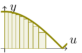
Figure 4.4: Integrating the cosine curve
The graphs look similar; the heights of the rectangles are the same, but the change of variable is distorting the base lengths, so if we were simply to integrate \(\sqrt{1-\sin^2u}\) with respect to \(u\), we would get the wrong answer.
However, we know that \(\delta x\approx\frac{dx}{du}\delta u\), so we can see that the base lengths of our rectangles are being stretched by \(\frac{dx}{du}\). As \(f(x)=f(x(u))\), we have that the rectangle under \(f(x)\) has area \[f(x)\delta x\approx f(x(u))\frac{dx}{du}\delta u.\] Adding up all these rectangles, and letting the widths approach \(0\), gives the result \[\int f(x)\,dx=\int f(x(u))\frac{dx}{du}\,du,\] which is integration by substitution.
For functions of two variables, integration will represent something rather similar; it will mean the volume under a surface \(z=f(x,y)\). We approximate the volume by summing the volumes of the cuboids of base widths \(\delta x\times\delta y\) and height \(f(x,y)\).
We will want to apply a change of variable \(x=x(u,v)\), \(y=y(u,v)\), and consider the integral of \(f(x,y)\) after making the substitutions. The base of the cuboid is a rectangle of size \(\delta x\,\delta y\).
It will turn out that we can write \(\begin{pmatrix}\delta x\\\delta y\end{pmatrix}\) as \(M\begin{pmatrix}\delta u\\\delta v\end{pmatrix}\) for some matrix \(M\).
The observation above shows that the area \(\delta x\,\delta y\) is then scaled by the determinant \(\det M\) of the matrix. So it is this determinant which plays the same role of the scaling factor in the two-variable integral as the differential \(\frac{dx}{du}\) plays in the one-variable case. We will see more later!
4.2 \(3\times3\) determinants
4.2.1 Definition
Consider 3 equations in 3 variables, \(A\mathbf{x}=\mathbf{b}\): \[\begin{aligned} ax+by+cz=j\\ dx+ey+fz=k\\ gx+hy+iz=l\end{aligned}\] If you try to solve this system, and eliminate each variable in turn, you will find that the algebraic expressions for \(x\), \(y\) and \(z\) all have the denominator \[aei-afh+bfg-bdi+cdh-ceg.\] So if this number is non-zero, the equations will have a unique solution. This is the determinant of the \(3\times3\)-matrix \[A=\begin{pmatrix} a&b&c\\ d&e&f\\ g&h&i \end{pmatrix}.\]
Rearranging, we have \[a(ei-fh)-b(di-fg)+c(dh-eg).\] Note that \((ei-fh)\), \((di-fg)\), and \((dh-eg)\) are second-order determinants left in \[\det A=\begin{vmatrix} a&b&c\\ d&e&f\\ g&h&i \end{vmatrix}\] when the row and column containing \(a\), \(b\) and \(c\) respectively are deleted. These determinants are called minors of \(a\), \(b\) and \(c\). So the minor corresponding to the element \(b\), say, is got by removing the row and column involving \(b\): \[\begin{vmatrix} \bullet&\bullet&\bullet\\ d&\bullet&f\\ g&\bullet&i \end{vmatrix}=\begin{vmatrix}d&f\\g&i\end{vmatrix}.\] As you can see from the expression above, we form the determinant by going along the top row, multiplying each element by its corresponding minor, and taking the alternating sum.
The sign to be attached to each product is formed from the row of alternating signs \[\begin{vmatrix} +&-&+\\ -&+&-\\ +&-&+ \end{vmatrix}.\] Notice that we have a \(+\) symbol if \(i\) and \(j\) add to an even number and a \(-\) symbol if they add to an odd number: a simple formula for this sign is \((-1)^{i+j}\). We define the cofactor of the \(ij\)th element of the matrix as \((-1)^{i+j}\) multiplied by the minor, so that the cofactor of \(a\) is defined as \[+\begin{vmatrix} e&f\\ h&i \end{vmatrix}=ei-fh.\] The cofactor of \(b\) is defined as \[-\begin{vmatrix} d&f\\ g&i \end{vmatrix}=-(di-fg).\] The cofactor of \(c\) is defined as \[+\begin{vmatrix} d&e\\ g&h \end{vmatrix}=dh-eg.\]
As already noted, the expression above shows that \[\det A=a\times(\mbox{cofactor of $a$})+b\times(\mbox{cofactor of $b$})+c\times(\mbox{cofactor of $c$}).\] That is, we go along the top row of \(A\), and take the products of each element with its cofactor, and take the sum of these, then this gives the determinant.
Remarkably, if we select any row or column, exactly the same happens. For each entry in the matrix, its cofactor is the determinant of the matrix with the row and column of the entry removed. Then the determinant is got by taking the sum of each matrix element multiplied by its cofactor (remember the alternating signs in the definition of the cofactor).
For example, if we take the middle column, with elements \(b\), \(e\) and \(h\), we note that \[\det A=-b(di-fg)+e(ai-cg)-h(af-cd),\] and this can be written \[b\times(\mbox{cofactor of $b$})+e\times(\mbox{cofactor of $e$})+h\times(\mbox{cofactor of $h$}).\]
This example was evaluated by expanding by the top row. As we noted already, a determinant may be expanded along any of its rows or any of its columns; the signs are as already indicated.
Example 4.3 Let’s work out \[\begin{vmatrix} 1&2&4\\ 3&1&-1\\ 2&5&6 \end{vmatrix}\] by expanding by the first column.
\[1\begin{vmatrix} 1&-1\\ 5&6 \end{vmatrix}-3\begin{vmatrix} 2&4\\ 5&6 \end{vmatrix}+2\begin{vmatrix} 2&4\\ 1&-1 \end{vmatrix}=1\times 11-3\times(-8)+2 \times(-6)=23\]Try for yourself, expanding along another row or column.
4.2.2 Vectors
This is really a part of MAS112, so this isn’t examinable in this module. But most of you are doing MAS112, or have seen it at A-level, and it will allow us to make more sense of \(3\times3\)-determinants. We quickly review some properties.
We’ve already seen the idea of a vector, \(\mathbf{v}=\begin{pmatrix}a\\b\\c\end{pmatrix}\), and we add these in the usual way.
Given two vectors, \(\mathbf{v}=\begin{pmatrix}a\\b\\c\end{pmatrix}\) and \(\mathbf{w}=\begin{pmatrix}d\\e\\f\end{pmatrix}\), there are two products we can make:
The dot product, or scalar product
We form the dot product, or scalar product, \(\mathbf{v}.\mathbf{w}=ad+be+cf\); this is a number, and has the property that \(\mathbf{v}.\mathbf{w}=|\mathbf{v}||\mathbf{w}|\cos\theta\), where \(\theta\) is the angle in between the two vectors.
So \[\begin{pmatrix}1\\2\\3\end{pmatrix}\cdot\begin{pmatrix}4\\5\\6\end{pmatrix}=1\times4+2\times5+3\times6=32.\] Since the length of \(\begin{pmatrix}1\\2\\3\end{pmatrix}\) is \(\sqrt{1^2+2^2+3^2}=\sqrt{14}\), and similarly the length of \(\begin{pmatrix}4\\5\\6\end{pmatrix}\) is \(\sqrt{4^2+5^2+6^2}=\sqrt{77}\), we can read off the cosine of the angle between them with the equation \(32=\sqrt{14}.\sqrt{77}\cos\theta\).
Two vectors at right-angles have dot product equal to \(0\).
Actually, we’ve already seen the dot product – it is just the matrix product \[\begin{pmatrix}1&2&3\end{pmatrix}\begin{pmatrix}4\\5\\6\end{pmatrix}.\] Although you are likely to meet dot products like this first in 3 dimensions, everything makes perfect sense in any number of dimensions when formulated like this in terms of a matrix product, and all the results mentioned continue to hold.
The cross product, or vector product
We can also form the cross product, or vector product, defined by \[\mathbf{v}\times\mathbf{w}=\begin{pmatrix}a\\b\\c\end{pmatrix}\times\begin{pmatrix}d\\e\\f\end{pmatrix}=\begin{pmatrix}bf-ce\\cd-af\\ae-bd\end{pmatrix};\] notice that this is a vector, and each component looks like a \(2\times2\)-determinant. This has the following properties:
\(|\mathbf{v}\times\mathbf{w}|=|\mathbf{v}||\mathbf{w}|\sin\theta\); in particular, this means that this is exactly the area of the parallelogram generated by \(\mathbf{v}\) and \(\mathbf{w}\);
\(\mathbf{v}\times\mathbf{w}\) is orthogonal to both \(\mathbf{v}\) and \(\mathbf{w}\);
\(\mathbf{v}\), \(\mathbf{w}\), \(\mathbf{v}\times\mathbf{w}\) forms a right-handed system.
As an example, \[\begin{pmatrix}1\\2\\3\end{pmatrix}\times\begin{pmatrix}4\\5\\6\end{pmatrix}=\begin{pmatrix}2\times6-3\times5\\3\times4-1\times6\\1\times5-2\times4\end{pmatrix}=\begin{pmatrix}-3\\6\\-3\end{pmatrix}.\]
(Note that if we set \(c=f=0\), so that \(\mathbf{x}\) and \(\mathbf{y}\) lie in the \(x\)-\(y\) co-ordinate plane, then \(\mathbf{x}\times\mathbf{y}=(0,0,ae-bd)\) has length clearly equal to \(ae-bd\), a \(2\times2\)-determinant, and we’ve already seen that this is the area of the parallelogram generated by \(\mathbf{x}\) and \(\mathbf{y}\); since it points in the \(z\)-direction, it is clearly orthogonal to both \(\mathbf{x}\) and \(\mathbf{y}\).)
If we write \(\mathbf{i}=(1,0,0)\), \(\mathbf{j}=(0,1,0)\) and \(\mathbf{k}=(0,0,1)\), as is usual, we see that \[\mathbf{x}\times\mathbf{y}=(bf-ce)\mathbf{i}+(cd-af)\mathbf{j}+(ae-bd)\mathbf{k},\] and a simple comparison with the formula for a \(3\times3\)-determinant shows that \[\mathbf{x}\times\mathbf{y}=\begin{vmatrix}\mathbf{i}&a&d\\\mathbf{j}&b&e\\\mathbf{k}&c&f\end{vmatrix},\] so this vector product can also be viewed as a \(3\times3\)-determinant.
4.2.3 Determinants as volumes
We’ve already seen that a \(2\times2\) determinant can be viewed as the area of a parallelogram, and it might not then come as too much of a surprise that something similar happens in three dimensions. So, given three vectors, \[\mathbf{u}=\begin{pmatrix}a\\b\\c\end{pmatrix},\quad \mathbf{v}=\begin{pmatrix}d\\e\\f\end{pmatrix},\quad \mathbf{w}=\begin{pmatrix}g\\h\\i\end{pmatrix},\] we can form the shape bounded by combinations of these vectors, a parallelepiped.

Figure 4.5: A parallelepiped
It may be possible to work out its volume in the same way as above, taking a cuboid and cutting bits out. But it’s probably easier here to use some vector notation. So that’s what we’ll do.
The two vectors \(\mathbf{u}\) and \(\mathbf{v}\) generate a parallelogram, whose area is \(|\mathbf{u}\times\mathbf{v}|\).

Figure 4.6: The base of the parallelepiped
To work out the volume of the parallelepiped generated by \(\mathbf{u}\), \(\mathbf{v}\) and \(\mathbf{w}\), we simply need to multiply this base area by the height. But this height is given by the projection of \(\mathbf{w}\) onto a line perpendicular to \(\mathbf{u}\) and \(\mathbf{v}\) – i.e., onto \(\mathbf{u}\times\mathbf{v}\).

Figure 4.7: The normal to the base added
The length of the projection is given by \(|\mathbf{w}|\cos\phi\), where \(\phi\) is the angle between \(\mathbf{w}\) and \(\mathbf{u}\times\mathbf{v}\).

Figure 4.8: Calculating the volume of the parallelepiped
Since the area of the base is \(|\mathbf{u}\times\mathbf{v}|\), it is easy now to see that the volume of the parallelepiped is given by the dot product of \(\mathbf{u}\times\mathbf{v}\) and \(\mathbf{w}\), which is (using the formula for the cross product above): \[\begin{eqnarray*} \mathbf{u}\times\mathbf{v}.\mathbf{w}&=&(bf-ce,cd-af,ae-bd).(g,h,i)\\ &=&(bf-ce)g+(cd-af)h+(ae-bd)i\\ &=&\begin{vmatrix}a&d&g\\b&e&h\\c&f&i\end{vmatrix}.\end{eqnarray*}\] Thus we can see that the determinant is exactly the volume of the parallelepiped, as we claimed.
4.3 General determinants
4.3.1 Higher order determinants
These ideas extend to higher order determinants, and a lot of arithmetic tends to be involved. Luckily, computers can do this easily. But maybe everyone should try a \(4\times4\)-determinant once in their lives! To illustrate the method, we’ll take a \(4\times4\)-determinant, and reduce it to a computation of several \(3\times3\)-determinants (which you can do yourself, if you are feeling bored).
Example 4.4 \[\begin{vmatrix} 1&3&4&2\\ 2&4&1&7\\ 0&3&2&-2\\ 1&1&3&-1 \end{vmatrix}=1\begin{vmatrix} 4&1&7\\ 3&2&-2\\ 1&3&-1 \end{vmatrix}-3\begin{vmatrix} 2&1&7\\ 0&2&-2\\ 1&3&-1 \end{vmatrix}+4\begin{vmatrix} 2&4&7\\ 0&3&-2\\ 1&1&-1 \end{vmatrix}-2\begin{vmatrix} 2&4&1\\ 0&3&2\\ 1&1&3 \end{vmatrix},\] by expanding along the top row. (Note again the alternating signs.)
Think about why there might have been better choices of rows or columns to choose.4.3.2 General properties of determinants
The determinant of the transpose is the same as the original determinant.
Again, \[\begin{vmatrix} a&b\\ c&d \end{vmatrix}=ad-bc=\begin{vmatrix} a&c\\ b&d \end{vmatrix}.\]
Interchanging two rows or columns multiplies the determinant by \(-1\).
As an example, consider \[\begin{vmatrix} a&b\\ c&d \end{vmatrix}=ad-bc.\] Now interchange rows 1 and 2: \[\begin{vmatrix} c&d\\ a&b \end{vmatrix}=cb-da=-(ad-bc).\]
If we add a multiple of one row to another, the determinant is unchanged. Again, let’s consider \(\begin{pmatrix} a&b\\ c&d \end{pmatrix}\), and form \(R_2\to R_2+\lambda R_1\). Then we get the determinant \[\begin{vmatrix} a&b\\ c+\lambda a&d+\lambda b \end{vmatrix}=a(d+\lambda b)-b(c+\lambda a)=ad-bc.\]
If we scale one row or one column by a scalar \(k\), then the determinant is multiplied by \(k\). For example, \[\begin{vmatrix} ka&kb\\ c&d \end{vmatrix}=kad-kbc=k(ad-bc)=k\begin{vmatrix} a&b\\ c&d \end{vmatrix}.\]
If the whole \(n\times n\)-matrix is scaled by a factor \(k\), then the determinant is multiplied by \(k^n\). Of course, this is just a special case of the last one, applied to each row in turn. We can see this in a \(2\times2\) example: \[\begin{vmatrix} ka&kb\\ kc&kd \end{vmatrix}=ka.kd-kb.kc=k^2(ad-bc).\]
Determinants of upper triangular matrices are easy!
Consider the case of a \(3\times3\) determinant with zeros below the leading diagonal: \[\begin{vmatrix} a&b&c\\ 0&e&f\\ 0&0&i \end{vmatrix}.\] We can make life easy for ourselves by expanding down the first column: \[a\begin{vmatrix} e&f\\ 0&i \end{vmatrix}-0\begin{vmatrix} b&c\\ 0&i \end{vmatrix}+0\begin{vmatrix} b&c\\ e&f \end{vmatrix},\] and we see that we don’t need to work out two of the determinants, since they get multiplied by \(0\). So we simply get \[a\begin{vmatrix} e&f\\ 0&i\end{vmatrix}=aei.\] In general, expanding down the first column will give only one term which may be non-zero, since all the other terms will vanish, and then the cofactor is also upper triangular (but of smaller size), so the same thing happens again.
You should be able to convince yourself that the determinant of an upper triangular matrix is just the product of the diagonal entries.
Lower triangular matrices work in the same way as upper triangular matrices. And diagonal matrices are examples of both, so they also have the property that their determinant is the product of their diagonal entries.
As the identity matrix is a diagonal matrix with \(1\)s along the diagonal, we see that \(\det I=1\). (This should hopefully be clear anyway, since multiplying by \(I\) keeps everything fixed, and so won’t change any areas/volumes etc.)
Properties (2), (3) and (4) explain how the determinant changes under all our elementary row operations. This last result suggests another easy way to evaluate \(3\times3\) (and larger) determinants: use row operations to reduce the matrix to upper triangular form, and then simply take the product of the diagonal entries, as suggested by (6).
If in this process we produce a row or column (rows or columns) which is all zero, then \(\det A=0\). Remember that we can do this precisely if the rows (or columns) are linearly dependent.
4.3.3 Linear dependence and independence
We can test for linear independence or dependence of vectors by forming the determinant containing of these vectors as columns. For example:
4.3.4 Adjoint Matrix
Given a square matrix \(A\), its adjoint (\(\mathrm{adj}\,A\)) is defined as the transpose of the matrix of cofactors. The cofactor of \(A_{ij}\) is essentially the determinant that one needs to multiply \(a_{ij}\) in the calculation of the determinant of \(A\).
For example, if \[A=\begin{pmatrix} 1&2&3\\ 1&3&5\\ 1&5&12 \end{pmatrix},\] then the cofactor of \(a_{11}\) is \(3(12)-5(5)=11\). Similarly, the cofactor of \(a_{12}\) is \(-[12-5]=-7\), and the cofactor of \(a_{13}\) is \(1(5)-3(1)=2\).
For the second row, the cofactor of \(a_{21}\) is \(-[2(12)-5(3)]=-9\), the cofactor of \(a_{22}\) is \(12-3=9\), and the cofactor of \(a_{23}\) is \(-(5-2)=-3\).
Finally, on the bottom row, the cofactor of \(a_{31}\) is \(10-9=1\), the cofactor of \(a_{32}\) is \(-(5-3)=-2\), and the cofactor of \(a_{33}\) is \(3-2=1\).
So the matrix of cofactors is \[\begin{pmatrix} 11&-7&2\\ -9&9&-3\\ 1&-2&1 \end{pmatrix}.\] The transpose of matrix of cofactors is \[\mathrm{adj}\,A=\begin{pmatrix} 11&-9&1\\ -7&9&-2\\ 2&-3&1 \end{pmatrix}.\]
One importance of the adjoint matrix comes in computing the inverse of a matrix. Indeed, notice that \[A.\mathrm{adj}\,A= \begin{pmatrix} 1&2&3\\ 1&3&5\\ 1&5&12 \end{pmatrix} \begin{pmatrix} 11&-9&1\\ -7&9&-2\\ 2&-3&1 \end{pmatrix} =\begin{pmatrix} 3&0&0\\ 0&3&0\\ 0&0&3 \end{pmatrix}=3I.\] Try to figure out why this is!
Essentially, the diagonal entries are got by taking each row of the matrix and multiplying by the cofactors – this calculation is exactly the same as the one giving the determinant of \(A\), expanding along each row in turn. In this example, \[\det A=1(36-25)-2(12-5)+3(5-3)=11-14+6=3.\] The other entries consist of the same calculation, but with one row of \(A\) replaced by one of the others, so this is computing the determinant of a matrix got from \(A\) by replacing one row by another; then the resulting matrix has two identical rows, so its determinant vanishes. Thus all the off-diagonal elements in the product are \(0\).
In general, it is true that \[A.\mathrm{adj}\,A=\det A.I,\] so that \[A^{-1}=\frac{\mathrm{adj}\,A}{\det A}.\]
4.3.5 Cramer’s formula
Cramer’s formula solves systems of linear equations. Here is the result, first in the case of \(2\times 2\)-matrices. Consider \[\begin{pmatrix} a&b\\ c&d \end{pmatrix}\begin{pmatrix} x\\ y \end{pmatrix}=\begin{pmatrix} e\\ f \end{pmatrix}.\]
Then the solution is got by replacing each column of the \(2\times2\)-matrix of coefficients with the column of constants, taking the determinant, and dividing by the determinant of the matrix of coefficients: \[\begin{aligned} x&=\begin{vmatrix}e&b\\f&d\end{vmatrix}\left/\begin{vmatrix}a&b\\c&d\end{vmatrix}\right.\\ y&=\begin{vmatrix}a&e\\c&f\end{vmatrix}\left/\begin{vmatrix}a&b\\c&d\end{vmatrix}\right.\end{aligned}\] if \(ad-bc\ne0\). This is an easy exercise (do it!).
But the result also generalises to the \(n\times n\) case. If \(A\mathbf{x}=\mathbf{b}\), where \[A=\begin{pmatrix} a_{11}&a_{12}&\ldots&a_{1n}\\ a_{21}&a_{22}&\ldots&a_{2n}\\ \vdots&\vdots&\ddots&\vdots\\ a_{n1}&a_{n2}&\ldots&a_{nn} \end{pmatrix},\; \mathbf{b}=\begin{pmatrix} b_1\\ b_2\\ \vdots\\ b_n \end{pmatrix},\] then \(x_k=\dfrac{\det A_k}{\det A}\) for \(k=1,\ldots,n\), if \(\det A\ne0\), where \(A_k\) is got by replacing the \(k\)th column of \(A\) with \(\mathbf{b}\): \[A_k=\begin{pmatrix} a_{11}&\ldots&b_1&\ldots&a_{1n}\\ a_{21}&\ldots&b_2&\ldots&a_{2n}\\ \ldots&\ldots&\ldots&\ldots&\ldots\\ a_{n1}&\ldots&b_n&\ldots&a_{nn} \end{pmatrix}\] with the \(k\)th column now equal to \(\mathbf{b}\).
4.3.6 Geometric meaning of \(\det A\)
We have already seen the geometric interpretation of \(\det A\) in the \(2\times2\) and \(3\times3\) case.
A parallelogram whose two sides are given by the two column vectors \(\begin{pmatrix} a\\ c \end{pmatrix}\) and \(\begin{pmatrix} b\\ d \end{pmatrix}\) has area equal to \(|\det A|\) where \(A=\begin{pmatrix}a&b\\c&d\end{pmatrix}\).
A parallelepiped whose three sides are given by the three column vectors \(\mathbf{a}=\begin{pmatrix}a_1\\a_2\\a_3\end{pmatrix}\), \(\mathbf{b}=\begin{pmatrix}b_1\\b_2\\b_3\end{pmatrix}\) and \(\mathbf{c}=\begin{pmatrix}c_1\\c_2\\c_3\end{pmatrix}\) has volume equal to \(|\det A|=|(\mathbf{a}\times\mathbf{b}).\mathbf{c}|\).
In higher dimensions, we have exactly the same result – the determinant measures the volume (in a suitable \(n\)-dimensional sense) of the parallelepiped spanned by the columns of the matrix.
Again, as we mentioned in the 2-dimensional case, these columns are exactly the result of applying the matrix to the standard set \[\begin{pmatrix}1\\0\\0\\\vdots\\0\end{pmatrix},\quad\begin{pmatrix}0\\1\\0\\\vdots\\0\end{pmatrix},\ldots,\begin{pmatrix}0\\0\\0\\\vdots\\1\end{pmatrix}.\] Again, we conclude that the determinant measures the factor by which volumes are scaled by multiplication by the matrix.
4.3.7 The multiplicative property of determinants
Perhaps the most useful result about determinants is the following:
For any square matrices \(A\) and \(B\) we have \[\det(AB)=\det A.\det B.\]
This is easy to verify by hand in the case of \(2\times2\)-matrices: if \[A=\begin{pmatrix}a&b\\c&d\end{pmatrix},\;B=\begin{pmatrix}e&f\\g&h\end{pmatrix},\] we have \(\det A=ad-bc\), \(\det B=eh-fg\). Now \[AB=\begin{pmatrix}a&b\\c&d\end{pmatrix}\begin{pmatrix}e&f\\g&h\end{pmatrix}=\begin{pmatrix}ae+bg&af+bh\\ce+dg&cf+dh\end{pmatrix}.\] Then \[\begin{aligned} \det(AB)&=(ae+bg)(cf+dh)-(af+bh)(ce+dg)\\ &=aecf+aedh+bgcf+bgdh-afce-afdg-bhce-bhdg\\ &=ad(eh-fg)+bc(gf-he)\\ &=(ad-bc)(eh-fg)\\ &=\det A.\det B,\end{aligned}\] as claimed.
However, if you are willing to accept the above statement that the determinant measures the factor by which volumes change on multiplying by the matrix, then the result should be clear, since we defined the product \(AB\) in terms of first multiplying a vector by \(B\) and then by \(A\); the first multiplication scales volumes by a factor of \(\det B\), and the second by a factor of \(\det A\), so the total scale factor will be \(\det A.\det B\). On the other hand, this was how the product \(AB\) was defined, so the volume ought to increase by \(\det(AB)\).
As a corollary, we notice the following: