9 Integration of functions of a single variable

Partly in preparation for integration of functions of two variables, which we will consider in the next chapter, this chapter will examine the limiting process that defines integration. We will see how flexible the limiting process is. In particular, we will see that careful consideration of the limiting process allows us to write down formulas for arc lengths, and certain areas and volumes.

9.1 Integration as a limiting process

Recall that $\int_a^bf(x)\,dx$ is the limit as $\delta x\to0$ of the sum of $f(x_i)\delta x$, when the interval $[a,b]$ is broken into intervals $[x_i,x_{i+1}]$ of width $\delta x$, coming from measuring the area of the rectangles which approximate the area under the curve.

This definition is called the “Riemann sum” definition of the definite integral. Leaving the technical details aside, when we divide an interval $[a,b]$ into $n$ subintervals of length $\delta x=\tfrac{b-a}{n}$, given by $[x_{i-1},x_i]$, we define the definite integral by \[\begin{equation} \int_a^bf(x)\,dx=\lim_{n\rightarrow\infty}\sum_{i=1}^nf(x_i)\delta x \tag{9.1} \end{equation}\] if the limit of the sum exists.

Formally, this is the definition of the integral – the results of taking limits as $\delta x\to0$ of the sum. It is a theorem that for any “reasonable” function $f$, this value $\int_a^bf(x)\,dx$ works out the area under the curve.

The interpretation is that the sum on the right gives a good approximation of the area under the graph of a positive function $f(x)$ when $n$ is very large:

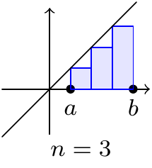
Figure 9.1: Approximating the area under a graph

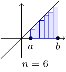
Figure 9.2: A better approximation

Figure 9.3: CAPTION

For a general function $f(x)$, the definite integral $\int_a^cf(x)\,dx$ gives a signed area. Namely, if $f(x)$ has a graph like the function below then \[\int^c_a f(x)~dx=A-B.\]

Figure 9.4: The signed area

The “theorem” mentioned above should seem natural. But be aware that strange functions exist!

Example 9.1 Let \[f(x)=\left\{ \begin{array}{cl} 0&\mbox{if $x$ is irrational}\\ 1&\mbox{if $x$ is rational} \end{array}\right.\] Think about what the “theorem” ought to say about this function! The natural divisions of $[0,1]$ are at the rational numbers $\frac{i}{n}$, so all the values will be $1$ at these points, and every sum will be $1$.

However, randomly chosen numbers between $0$ and $1$ will be irrational (irrationals are uncountable, rationals are countable), so that most values taken by $f$ are $0$, and the “right” answer for the area should be $0$.

In practice, we (just about) never use integration by first principles. Instead, we use the Fundamental Theorem of Calculus, which says that differentiation and integration are inverse. The following is a precise statement of the Fundamental Theorem of Calculus for a continuous function $f(x)$:

Theorem 9.1 (The Fundamental Theorem of Calculus) Let $f(x)$ be a continuous function on the interval $[a,b]$. The function $F(x)$ defined on $[a,b]$ by \[F(x)=\int_a^xf(t)\,dt\] is differentiable at $x$ and $F'(x)=f(x)$.

When $f(t)$ is continuous, we really can regard $\int_a^xf(t)\,dt$ as the area under the curve between $a$ and $x$. So: \[\begin{aligned} F(x)&=\mbox{area under $f$ between $a$ and $x$};\\ F(x+\delta x)&=\mbox{area under $f$ between $a$ and $x+\delta x$};\\ F(x+\delta x)-F(x)&=\mbox{area under $f$ between $x$ and $x+\delta x$}.\end{aligned}\]

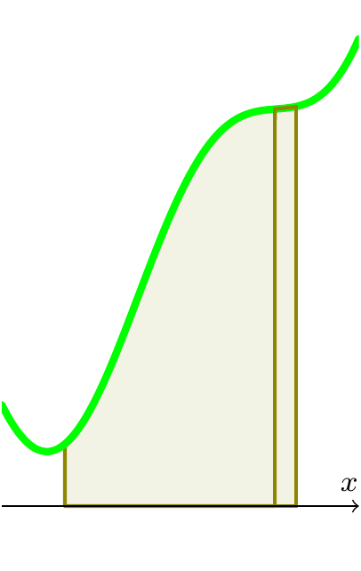
Figure 9.5: Justification for the Fundametal Theorem of Calculus

We recall that \[F'(x)=\lim_{\delta x\to0}\frac{F(x+\delta x)-F(x)}{\delta x}.\] If $\delta x$ is small, $f(t)$ will not change much between $x$ and $x+\delta x$, so the area under $f$ between $x$ and $x+\delta x$ is well approximated by a rectangle of width $\delta x$ and height $f(x)$.

Figure 9.6: The area of a rectangle

So $F(x+\delta x)-F(x)\approx f(x)\delta x$. So $F'(x)=f(x)$.

Think about this argument carefully, and what you might need to do to make it more rigorous!

Example 9.2 We know that $\frac{d}{dx}x^n=nx^{n-1}$ and that $\int_a^bx^ndx=\frac{1}{n+1}\left(b^{n+1}-a^{n+1}\right)$, from first principles. So for $f(x)=x^2$, the function $F(x)$ given by \[F(x)=\int_a^xf(t)~dt=\int_a^xt^2dt=\left[\frac{1}{3}t^3\right]_{t=a}^{t=x}=\tfrac13x^3-\tfrac{1}{3}a^3\] has \[F'(x)=\frac{d}{dx}\left(\tfrac{1}{3}x^3-\tfrac{1}{3}a^3\right)=x^2=f(x)\] as expected.

Example 9.3 We can calculate the derivative of the function \[I(x)=\int_0^{x^2}e^{t^2}~dt\] using the Fundamental Theorem of Calculus. The function $I(x)=f(g(x))$ where \[f(x)=\int_0^xe^{t^2}~dt\qquad \text{ and }\qquad g(x)=x^2.\] The chain rule tells us that \[\frac{dI}{dx}=\frac{df}{dg}\frac{dg}{dx}=e^{(x^2)^2}2x=2x\,e^{x^4}\] where the derivative $\frac{df}{dg}$ is calculated using Theorem 9.1.

In the following sections we will see how the idea of taking the limit of appropriate sums can be used to find arc lengths, surface areas, and volumes of various sorts.

9.2 More areas and volumes as limits

In this section we continue to explore the limiting process of integration of functions of a single variable to compute areas.

However, we start with a standard example of how we can use integration to find the area under the graph of a function.

Example 9.4 In this example we will show that the area of a disc of radius $R$ is $\pi R^2$. The disc centred at the origin of radius $R$ is bounded by the circle determined by $x^2+y^2=R^2$. The area of the upper half disc $U$ is therefore \[\text{area}(U)=\int_{-R}^{R}\sqrt{R^2-x^2}~dx.\] Setting $x=R\sin u$, so that $dx=R\cos u\,du$, we see that \[\begin{aligned} \text{area}(U)&=\int_{\arcsin(-1)}^{\arcsin(1)}\sqrt{R^2-(R\sin u)^2}~R\cos u~du=R^2\int_{-\frac{\pi}{2}}^{\frac{\pi}{2}}\sqrt{(1-\sin^2u)}~\cos u~du\\ &=R^2\int_{-\frac{\pi}{2}}^{\frac{\pi}{2}}\cos^2u~du=\frac{R^2}{2}\int_{-\frac{\pi}{2}}^{\frac{\pi}{2}}\cos(2u)+1~du=\frac{R^2}{2}\left[\frac{\sin(2u)}{2}+u\right]_{-\frac{\pi}{2}}^{\frac{\pi}{2}}\\ &=\frac{\pi R^2}{2}. \end{aligned}\] So the area of the disc $D$ of radius $R$ is \[\text{area}(D)=2\times\text{area}(U)=\pi R^2.\]

Reminding ourselves that integration is just a limiting operation, here is another way to calculate the area of a disc. Rather than having the sum of rectangles in mind, we can be more creative, and add up other shapes.

Example 9.5 Consider the picture:

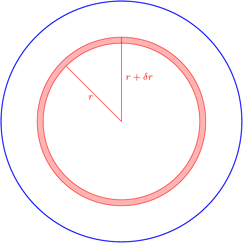
Figure 9.7: The circle as a union of annuli

To get the area of the disc, we add up the areas of the rings (“annuli”) of inner radius $r$ and outer radius $r+\delta r$. So the width of each annulus is $\delta r$. The area is approximately the circumference $2\pi r$ multiplied by the width (and this approximation looks better and better as $\delta r\to0$), so is about $2\pi r\,\delta r$. Splitting the radius into annuli with inner radius $r_{i-1}$ and outer radius $r_i=r_{i-1}+\delta r$, we get an approximation of $\sum_{i=1}^n2\pi r_i\,\delta r$ for the area, and as $\delta r\to0$, the limit is defined to be \[\int_0^R2\pi r\,dr=\pi R^2.\]

We now use some of the algebra that we have learnt to calculate the area bounded by an ellipse.

Example 9.6 Recall that if $L_A:\mathbb{R}^2\rightarrow\mathbb{R}^2$ is a map given by multiplication by a $2\times2$ matrix $A$, \[\begin{pmatrix}x\\y\end{pmatrix}\mapsto\begin{pmatrix}a_{11}&a_{12}\\a_{21}&a_{22}\end{pmatrix}\begin{pmatrix}x\\y\end{pmatrix}=\begin{pmatrix}a_{11}x+a_{12}y\\ a_{21}x+a_{22}y\end{pmatrix},\] and $D\subseteq\mathbb{R}^2$ then $\text{area}(L_A(D))=\det(A)\text{area}(D)$.

For the matrix $A=\begin{pmatrix}a&0\\0&b\end{pmatrix}$ and $D=\{(x,y)~|~x^2+y^2\leq1\}$ the unit disc, the points in $L_A(D)$ are points $(u,v)=(ax,by)$ that satisfy $x^2+y^2\le1$. That is \[L_A(D)=\left\{(u,v)~\left|~\frac{u^2}{a^2}+\frac{v^2}{b^2}\le1\right.\right\}.\] So $L_A(D)$ is the region bounded by the standard form of an ellipse $\mathcal{E}$ with major/minor axes $a$ and $b$. This means \[\text{area bounded by }\mathcal{E}=\text{area}(L_A(D))=\det(A)\text{area}(D)=\pi ab.\]

Notice that the area $A$ of a circle of radius $r$ is $\pi r^2$, and the circumference is $C=2\pi r$. Observe that $\frac{dA}{dr}=C$. When you think about how the area changes as you move from a circle of radius $r$ to $r+\delta r$, you can see (look at the pictures!) that we are just adding an annulus of inner radius $r$ and outer radius $r+\delta r$. Clearly this is like adding a small rectangle of width $\delta r$ and length $C$. So you should be able to convince yourself that $\frac{dA}{dr}=C$, and see that the idea ought to generalise more – for spheres, for example, if we differentiate the formula for the volume, we ought to get the formula for the surface area.

For another example of computing areas in more creative ways than simply adding rectangles, we’ll prove, as an aside, a Pizza Theorem! We first need a simple lemma.

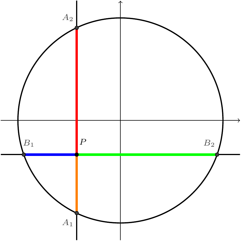
Lemma 9.1 Consider a circle of radius $r$ centred at $(0,0)$, and a point $P=(a,b)$ in the interior of the circle. Let $A_1$ and $A_2$ denote the two points of intersection of the line $x=a$ with the circle, and $B_1$ and $B_2$ denote the two points of interection of the line $y=b$ with the circle. Then the sum \[|PA_1|^2+|PA_2|^2+|PB_1|^2+|PB_2|^2\] is equal to $4r^2$, independent of $(a,b)$.

Proof. Here is a picture:

Figure 9.8: Diagram for the lemma

The coordinates of $A_1$ and $A_2$ are $(a,-\sqrt{r^2-b^2})$ and $(a,\sqrt{r^2-b^2})$; the coordinates of $B_1$ and $B_2$ are $(-\sqrt{r^2-a^2},b)$ and $(\sqrt{r^2-a^2},b)$. So the quantity in the statement is \[(b-\sqrt{r^2-a^2})^2+(b+\sqrt{r^2-a^2})^2+(a-\sqrt{r^2-b^2})^2+(a+\sqrt{r^2-b^2})^2,\] and it is easy (using $(x-y)^2+(x+y)^2=2(x^2+y^2)$) to see that this equals \[2(b^2+(r^2-a^2))+2(a^2+(r^2-b^2))=4r^2,\] as claimed.

Now we turn to the theorem:

Theorem 9.2 (Pizza Theorem) Take a (perfectly circular and uniformly thin) pizza, and choose any point. Make four cuts at angles of $\frac{\pi}{4}$, making 8 slices of pizza. If two people take alternate slices, then they get exactly the same amount of pizza.

Proof. From the lemma, we see that if we take any point inside the pizza, and make two perpendicular cuts through it, the total sum of the squares of the lengths of the sides from the point to the edges is $4r^2$, where $r$ denotes the radius of the pizza.

Now we imagine rotating the perpendicular lines in the above picture by an angle of $\delta\theta$ around $P$: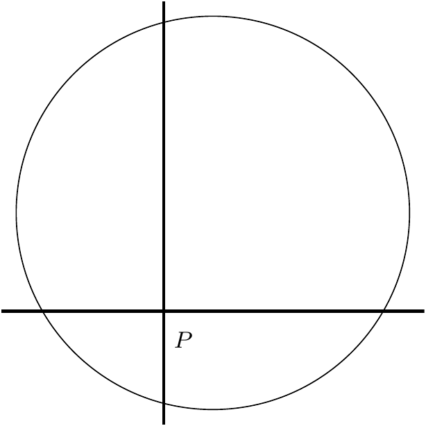

Figure 9.9: Cross shape

to get a picture:

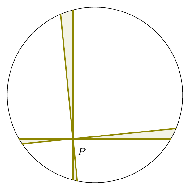
Figure 9.10: Diagram for the proof of the theorem

We approximate these very thin slices with isosceles triangles with angles $\delta\theta$. We recall that the area of an isosceles triangle with two sides of length $a$ and an angle of $\phi$ between these two sides is $\frac{1}{2}a^2\sin\phi$. So using the notation of the lemma, the total area of the four very thin slices is \[\tfrac{1}{2}|PA_1|^2\sin\delta\theta+\tfrac{1}{2}|PA_2|^2\sin\delta\theta+\tfrac{1}{2}|PB_1|^2\sin\delta\theta+\tfrac{1}{2}|PB_2|^2\sin\delta\theta,\] and the lemma tells us that this simplifies to $2r^2\sin\delta\theta$. Furthermore, since $\delta\theta$ is very small, this is approximately $2r^2\delta\theta$. You should be able to convince yourselves that these approximations become better and better as $\delta\theta\to0$.

Then if we rotate the first picture to create slices of an angle $\phi$, the area swept out is given by \[\int_0^\phi2r^2\,d\theta=2r^2\phi.\] In particular, if we sweep out an angle of $\frac{\pi}{4}$, to get four slices, the total area is $\frac{1}{2}\pi r^2$, and the other four slices, which make up the rest of the circle, must also have the same area, as required.

Notice that the same argument will work for any number of slices which is a multiple of $4$ which is at least $8$.

We now look at how this limiting process can be used to calculate volumes of cones.

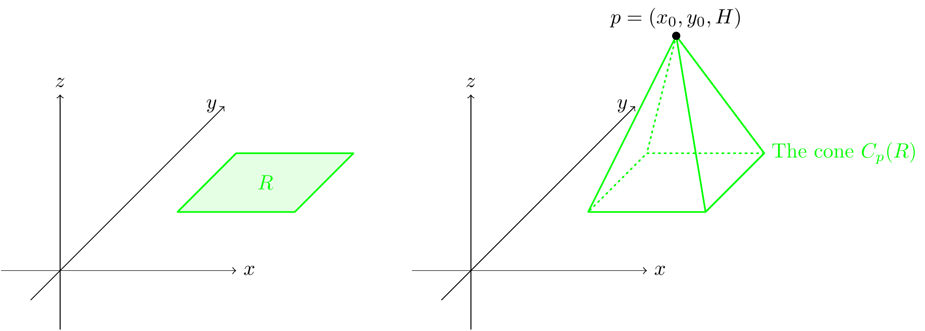
Example 9.7 Let $R$ be any region in the $xy$-plane and $p$ be any point in $\mathbb{R}^3$ of height $H$. We can form a cone $C_p(R)$ over this region by connecting all points on the boundary of $R$ to $p$. The diagram shows this process when $R$ is a quadrilateral, but the process works for any region.

Figure 9.11: A general cone

The volume of the cone $C_p(R)$ can be approximated using thin slices as in the picture (image taken from https://www.whitman.edu/mathematics/calculus_online/section09.03.html):

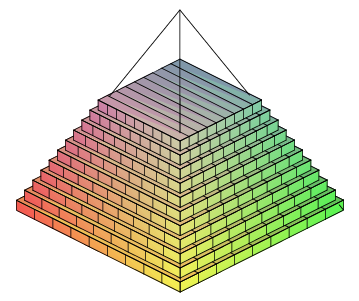
Figure 9.12: Splitting a pyramid into small chunks

\[\text{volume}(C_p(R))~\approx~\sum\text{thin slices}.\]

We will not be too precise here. However, in the limit of the approximation we find that the volume of the cone equals the integral of the areas of slices of the cone. So we only need to understand the area of the slices.

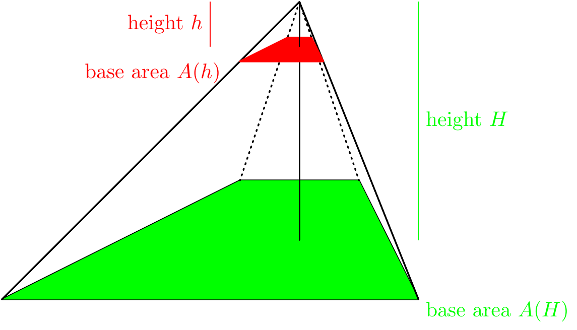
Figure 9.13: Understanding the volume of horizontal slices

From this picture, we see that the cone of height $h$ is similar to the cone of height $H$ with all side lengths of the larger cone being scaled by $\frac{h}H$. Thus \[A(h)=\left(\frac hH\right)^2A(H).\] But the volume of the cone is obtained by integrating the area of the slices. So \[\text{volume}\Big(C_p(R)\Big)=\int_{h=0}^H A(h)~dh=\int_{h=0}^H\left(\frac hH\right)^2A(H)~dh=\frac{A(H)}{H^2}\int_0^Hh^2~dh=\frac{A(H)H^3}{3}.\] The only thing we used about the point $P$ was that its height was $H$. Thus, we have shown that the volume of an arbitrary cone over a region $R$ of height $H$ is \[\frac{1}{3}\times\text{area}(R)\times H.\]

So for example, the area of a cone whose base is a circle of radius $r$ and whose height is $h$ is $\frac{1}{3}\pi r^2h$, as you probably know from school. But at school you might have seen this only for cones with circular base and axis which was perpendicular to the circle; the argument above generalises this to cones whose axis can be of any angle from the circle, and whose base is any shape at all!

Example 9.8 Again, we will not be too precise in this example (but you should try to convince yourself that it’s OK!). We will later see (Example 9.11) that the surface area of a sphere of radius $r$ is $4\pi r^2$. So as we integrate the areas of the sphere of radius zero to a sphere of radius $R$ we should get the volume of a ball of radius $R$. Namely: \[\begin{aligned} \text{volume}(\text{Ball of radius }R)&=\int_0^R\text{area}(\text{sphere of radius }r)~dr=\int_0^R4\pi r^2~dr\\ &=\left[\frac{4}{3}\pi r^3\right]_0^R=\frac{4}{3}\pi R^3.\end{aligned}\]

9.3 Arc length

In this section we will now use integration to find a very clean formula for the length of a curve $C=\{(x,f(x))\,|\,x\in[a,b]\}$ (just the graph of the function $f$) when $f(x)$ is differentiable. In particular, we will show that the length of $C$ is given by \[\begin{equation} \text{length}(C)=\int_a^b\sqrt{1+(f'(x))^2}~dx. \tag{9.2} \end{equation}\] To justify this formula, we firstly note that the length of $C$ can be approximated by the length of a curve consisting of line segments with vertices on the curve:

Figure 9.14: Arc length of a curve

Figure 9.15: Splitting the length into segments

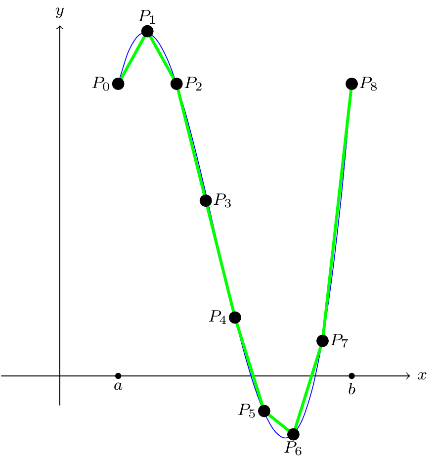
Figure 9.16: Splitting the length into more segments

The length of such a “polygonal approximation” $P$ to the curve $C$ improves as you add vertices, as the picture makes clear. So we make the following definition:

Definition 9.1 The length of a curve $C$ in the plane is the smallest number that is larger than the length of every polygonal approximation of $C$.

In most “reasonable” cases, the length of a curve will exist. However, “unreasonable" cases do exist (see the exercises for an example). Definition 9.1 also uses a deep property of the real numbers (see the”least upper bound" property below). We will now see that when the curve is the graph of a differentiable function that the length exists and is given by (9.2).

When we divide the interval $[a,b]$ into $n$ subintervals of length $\delta x$ we get a polygonal curve $\mathcal{P}_n$ with vertices $P_0,\dots,P_n$ with $P_k=(x_k,f(x_k))$ where $x_k=a+k\,\delta x$ and \[\text{length}(C)\approx\text{length}(\mathcal{P}_n)=\sum_{k=1}^{n}|P_{k-1}P_k|.\]

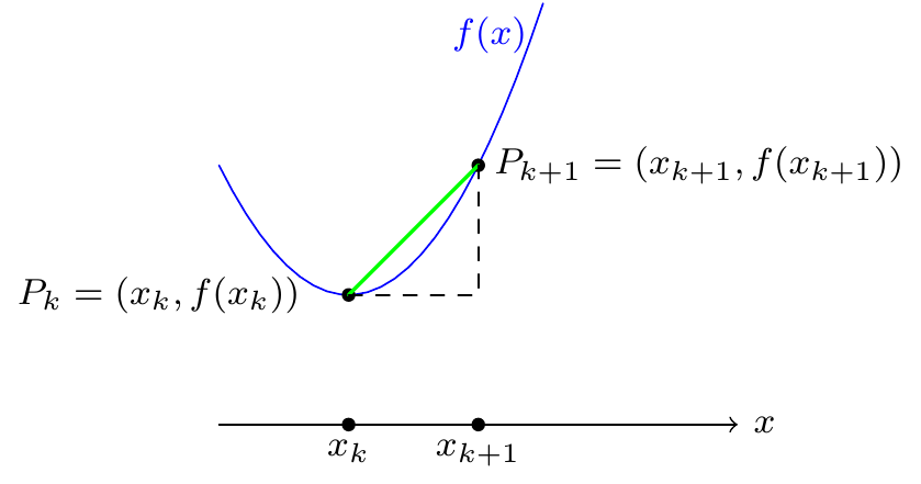
Figure 9.17: Length of a line segment

Looking at this picture, we see that the length $|P_kP_{k+1}|$ from $P_k$ to $P_{k+1}$ is given (using Pythagoras’s Theorem) by \[\begin{aligned} |P_kP_{k+1}|&=\sqrt{(x_k-x_{k+1})^2+(f(x_k)-f(x_{k+1}))^2}=\sqrt{\delta x^2+(f(x_k)-f(x_{k+1}))^2}\\ &=\delta x\sqrt{1+\left(\frac{f(x_k)-f(x_{k+1})}{\delta x}\right)^2}\\ &\approx\delta x\sqrt{1+f'(x_k)^2}\end{aligned}\] and that this approximation should look better and better as we take more and more $x_k$ values.

Then we have therefore shown that \[\sum_{k=1}^n|P_{k-1}P_k|\approx\sum_{k=1}^n\delta x\sqrt{1+f'(x_k)^2}.\] This gives us \[\text{length}(C)=\lim_{n\to\infty}\text{length}(\mathcal{P}_n)=\lim_{n\to\infty}\sum_{k=0}^n\delta x\sqrt{1+f'(x_k)^2}=\int_a^b\sqrt{1+\left(f'(x)\right)^2}\,dx\] where the last identity comes from Equation (9.1). Thus we have justified the following result:

Theorem 9.3 If $f(x)$ is a differentiable function on an interval $[a,b]$ then the length of the curve $C=\{(x,f(x))~|~x\in[a,b]\}$ is given by \[\textrm{length}(C)=\int_a^b\sqrt{1+(f'(x))^2}~dx.\]

In general, it is not easy to integrate this sort of expression. Here are a couple of examples where it does work (and others will be provided as exercises).

Example 9.9 Using Pythagoras’s Theorem, we know that the length of a straight line $l$ determined by the equation $y=mx+c$ between the points $(a,ma+c)$ and $(b,mb+c)$ is $\sqrt{(b-a)^2+(m(b-a))^2)}=(b-a)\sqrt{1+m^2}$. Using the formula from Theorem 9.3, we get \[\text{length}(l)=\int_a^b\sqrt{1+(y'(x))^2}~dx=\int_a^b\sqrt{1+m^2}~dx=\left[\left(\sqrt{1+m^2}\right) x\right]_a^b=(b-a)\sqrt{1+m^2}.\]

Now that we know that we get the correct length for a linear equation we look at the length of a quadratic equation.

Example 9.10 Let $P$ be the segment of the parabola $y=x^2$ over the interval $[a,b]$. We have \[\text{length}(P)=\int_a^b\sqrt{1+(y'(x))^2}~dx=\int_a^b\sqrt{1+4x^2}~dx.\] Using the substitution $x=\frac{1}{2}\sinh u$, so that $dx=\frac{1}{2}\cosh u\,du$, and the standard hyperbolic identity $\cosh^2u-\sinh^2u=1$, we get \[\begin{aligned} \text{length}(P)&=\frac{1}{2}\int_{\text{arcsinh}(2a)}^{\text{arcsinh}(2b)}\cosh u\sqrt{1+\sinh^2u}~du=\frac{1}{2}\int_{\text{arcsinh}(2a)}^{\text{arcsinh}(2b)}\cosh u\sqrt{\cosh^2u}~du\\ &=\frac{1}{2}\int_{\text{arcsinh}(2a)}^{\text{arcsinh}(2b)}\cosh^2u~dx.\end{aligned}\] Now we use the definition of $\cosh x$ in terms of exponentials: \[\cosh^2u=\left(\frac{e^u+e^{-u}}{2}\right)^2=\frac{e^{2u}+e^{-2u}+2}{4}=\frac{1}{2}\left(\cosh(2u)+1\right).\] So \[\text{length}(P)=\frac{1}4\int_{\text{arcsinh}(2a)}^{\text{arcsinh}(2b)}\cosh(2u)+1~du=\frac{1}4\left[\frac{1}2\sinh(2u)+u \right]_{\text{arcsinh}(2a)}^{\text{arcsinh}(2b)}.\] Using the definition of $\sinh x$ in terms of exponentials, we see: \[\sinh(2u)=\frac{e^{2u}-e^{-2u}}{2}=\frac{(e^u+e^{-u})(e^u-e^{-u})}{2}=2\cosh u.\sinh u=2\sqrt{1+\sinh^2u}\sinh u.\] So \[\begin{aligned} \text{length}(P)&=\frac{1}{4}\left[\frac{1}{2}\sqrt{1+\sinh^2u}\sinh(u)+u \right]_{\text{arcsinh}(2a)}^{\text{arcsinh}(2b)}\\ &=\frac{1}{8}\left(4b\sqrt{1+4b^2}-4a\sqrt{1+4a^2}+\text{arcsinh}(2b)-\text{arcsinh}(2a)\right).\end{aligned}\] If you wish to “simplify” this expression further, you can recall that $\text{arcsinh}\,y=\ln\left(y+\sqrt{y^2+1}\right)$.

9.4 Surface areas of revolution

In this section we will use integration to find a very clean formula for the area of a surface obtained by rotating a curve about the $x$-axis. In particular, we will show that when we rotate a curve $C=\{(x,f(x))~|~a\le x\le b\}$ about the $x$-axis that the area of the surface $S_C$ obtained has \[\begin{equation} \text{area}(S_C)=2\pi\int_a^b|f(x)|\sqrt{1+(f'(x))^2}~dx. \tag{9.3} \end{equation}\] To justify this formula, we firstly recall that a curve $C$ can be approximated by a polygonal curve $\mathcal{P}_n$ (as in the previous section). This means that we can approximate the surface of revolution $S_C$ by the surface obtained by rotating $\mathcal{P}_n$ about the $x$-axis. A polygonal approximation $\mathcal{P}_n$ of a curve $C=\{(x,f(x))~|~a\leq x\leq b\}$ consists of straight lines between adjacent vertices $(x_0,f(x_0)),(x_1,f(x_1)),\dots,(x_n,f(x_n))$ as above.

When we rotate a polygonal approximation $\mathcal{P}_n$ about the $x$-axis, the surface obtained is composed of pieces which are formed by rotating straight lines about the $x$-axis:

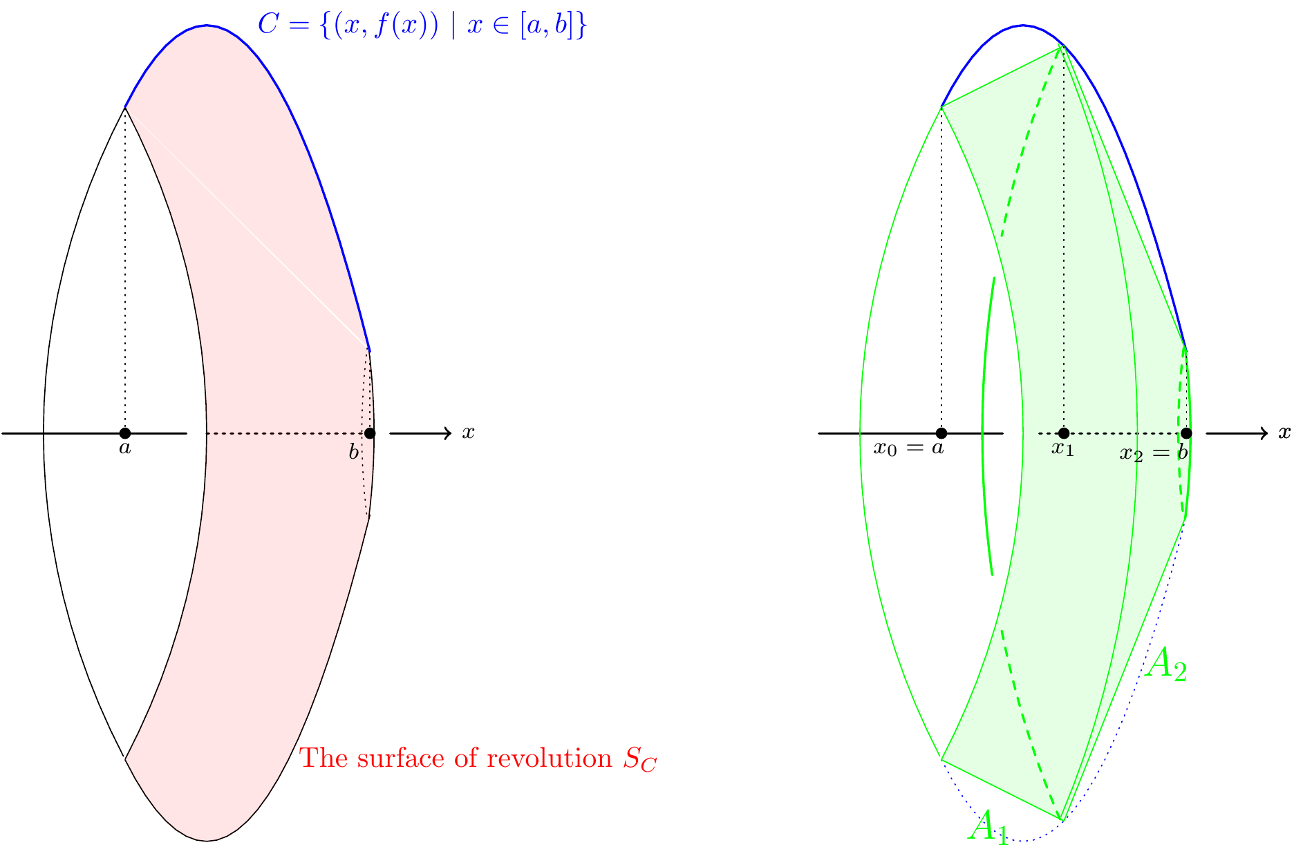
Figure 9.18: Rotating line segments

Each piece is called a frustum:

Figure 9.19: A frustum

So let’s work out the surface area of this frustum. We’ll argue slightly carelessly (which means that everything I say is going to be true, but perhaps a proper proof ought to contain more details…).

Essentially, we are rotating a line of length $l$ which is a radius $r_1$ from the origin. If the line were parallel to the axis of rotation, we’d have the surface of a cylinder, and you surely know that the surface area would be equal to the circumference $2\pi r$ of the circle, multiplied by the length of the line. But even if the line isn’t parallel to the axis, we will get the same result – so in fact, the surface area of the frustum is (approximately) $2\pi r_1l$, and as we take thinner and thinner slices, this becomes more and more accurate.

In practice, we are rotating part of an arc length, so we worked out $l$ in the previous section: $l=\sqrt{1+f'(x)^2}\delta x$. And the distance of this line segment from the axis is given by the value of the function, namely $f(x)$. However, note that if $f(x)<0$, then the distance is actually $-f(x)$; in fact, the distance we need is, in general, $|f(x)|$.

So we need to add up all the areas given by $2\pi|f(x)|\sqrt{1+f'(x)^2}\,\delta x$. The final result is:

Theorem 9.4 If $f(x)$ is a differentiable function on an interval $[a,b]$ then the area of the surface $S_C$ obtained by rotating the curve $C=\{(x,f(x))\,|\,x\in[a,b]\}$ about the $x$-axis is given by \[\mathrm{area}(S_C)=2\pi\int_a^b|f(x)|\sqrt{1+\left(f'(x)\right)^2}~dx.\]

We now illustrate how the formula can be used to calculate surface areas of solids of revolution with some examples.

Example 9.11 As an application of the formula, we calculate the area of a sphere of radius $r$. We know that the sphere of radius $r$ is obtained by rotating the graph of the function $f(x)=\sqrt{r^2-x^2}$ about the $x$-axis over the interval $[-r,r]$. So the surface area of the sphere of radius $r$ is \[\text{area}(\text{sphere of radius }r)=2\pi\int_{-r}^r|f(x)|\sqrt{1+\left(f'(x)\right)^2}~dx.\] In our case, we easily see that $f(x)\geq0$ on $[-r,r]$ and $f'(x)=-\frac x{\sqrt{r^2-x^2}}$. So \[\begin{aligned} \text{area}(\text{sphere of radius }r)&=2\pi\int_{-r}^r\sqrt{r^2-x^2}\sqrt{1+\left(-\frac x{\sqrt{r^2-x^2}}\right)^2}~dx\\ &=2\pi\int_{-r}^r\sqrt{r^2-x^2}\sqrt{\frac{(r^2-x^2)+x^2}{r^2-x^2}}~dx=2\pi r \int_{-r}^r~dx=4\pi r^2.\end{aligned}\]

Notice that if we were to put a cylinder around the sphere, parallel to the $x$-axis, it would go from $x=-r$ to $x=r$, and have radius $r$, so its surface area is given by $2\pi.r.(2r)$ (the usual formula for the area of a cylinder being $2\pi rh$ where $h$ denotes the height of the cylinder). So the surface area of the cylinder is equal to the surface area of the sphere. This beautiful result appears to have been known to Archimedes, and apparently a drawing of a cylinder circumscribing a sphere is said to have been drawn on his grave.

Looking at the proof in slightly more detail, we see something else rather lovely:

Theorem 9.5 (Tomato Theorem) The surface area of the slice of the sphere is proportional to the width of the slice.

So if you slice a (perfectly spherical) tomato into slices of equal width, then they contain exactly the same amount of skin.

Proof. We simply note that the surface area between $x=a$ and $x=b$ is now given by \[\begin{aligned} \text{area}&=2\pi\int_a^b\sqrt{r^2-x^2}\sqrt{1+\left(-\frac x{\sqrt{r^2-x^2}}\right)^2}~dx\\ &=2\pi\int_a^b\sqrt{r^2-x^2}\sqrt{\frac{(r^2-x^2)+x^2}{r^2-x^2}}~dx=2\pi r \int_a^b~dx=2\pi r(b-a).\end{aligned}\] So the area is indeed proportional to the width $(b-a)$.

The only other theorem I know named after food is the “Ham Sandwich Theorem”. This also involves volumes, but its proof is just a bit too far outside the course material. Basically it says that if you have three solid objects in 3-dimensional space, then there is a unique plane which cuts each of the objects into half (so each object has half of its volume on one side of the plane, and the other half on the other side). Think of a piece of ham inside two slices of bread – then there’s a unique slice through the sandwich which cuts both slices of bread and the ham into half.

Example 9.12 As a second example of calculating the area of a surface of revolution, we calculate the surface area of a paraboloid $P$ obtained by rotating the parabola given by the graph of $f(x)=x^{\frac{1}2}$ about the $x$-axis over the interval $[0,a]$. Again, clearly $f(x)\geq0$ on $[-r,r]$, and $f'(x)=\frac 1{2\sqrt{x}}$. So \[\begin{aligned} \text{area}(P)&=2\pi\int_0^a\sqrt{x}\sqrt{1+\left(\frac 1{2\sqrt{x}}\right)^2}~dx=2\pi\int_{0}^a\sqrt{x}\sqrt{\frac{4x+1}{4x}}~dx=2\pi\int_{0}^a\frac{\sqrt{x}}{\sqrt{4x}}\sqrt{4x+1}~dx\\ &=\pi\int_{0}^a\sqrt{4x+1}~dx=\left[\frac{\pi}4.\frac23(4x+1)^{\frac32}\right]_0^a=\frac{\pi}6\left((4a+1)^{\frac32}-1\right).\end{aligned}\]

9.5 Volumes of solids of revolution

A solid obtained by rotating a region bounded by the $x$-axis and a curve about the $x$-axis is called a solid of revolution.

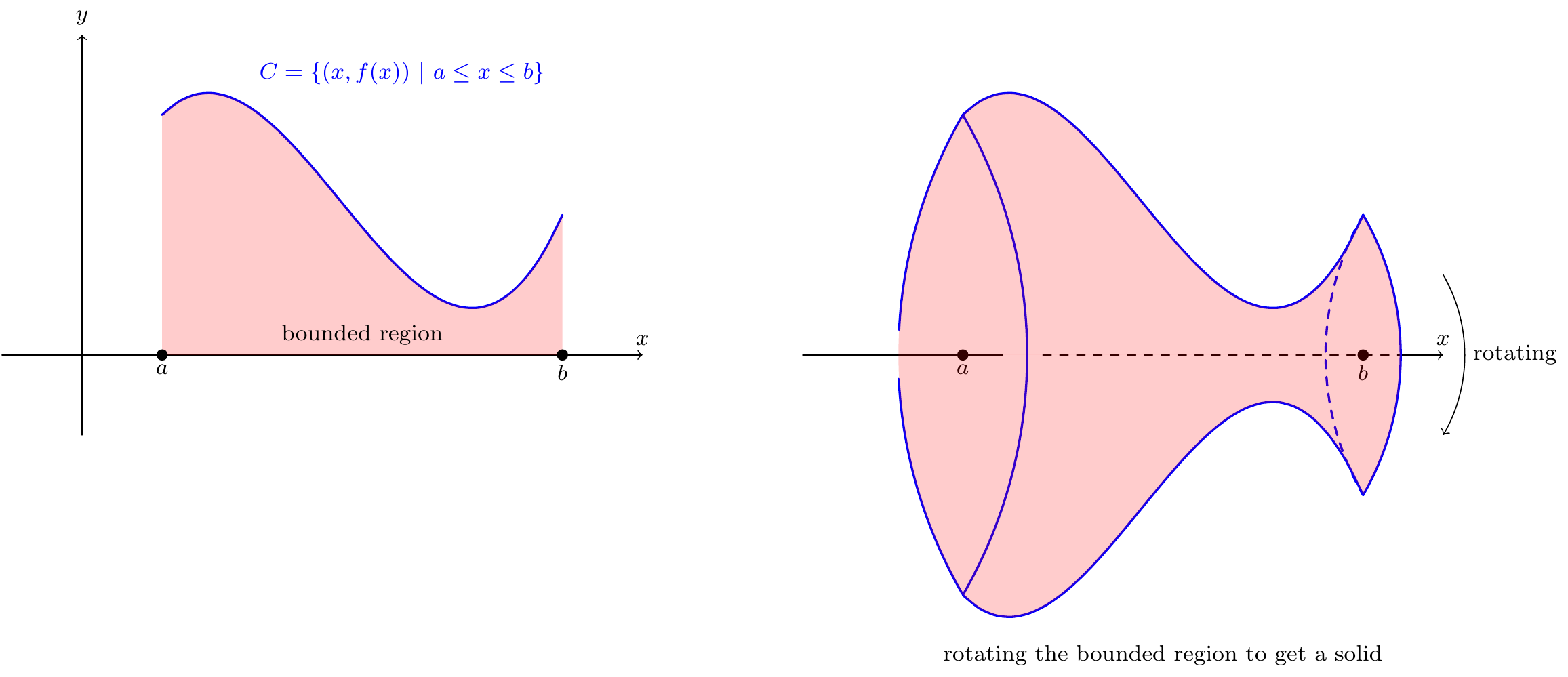
Figure 9.20: Rotating the area under a curve

In this section we will use a limiting process to find a formula for the volume of a solid of revolution. In particular, we will show that when we rotate the region bounded by $C=\{(x,f(x))~|~a\leq x\leq b\}$ about the $x$-axis that the volume of the solid $R_C$ obtained has volume \[\begin{equation} \text{vol}(R_C)=\pi\int_a^bf(x)^2~dx. \tag{9.4} \end{equation}\]

To justify this formula, we will consider the case when $f(x)>0$ on $[a,b]$. The volume of $R_C$ is equal to the sum of volumes of the thin slices $B_1,\dots,B_n$ in the picture below:

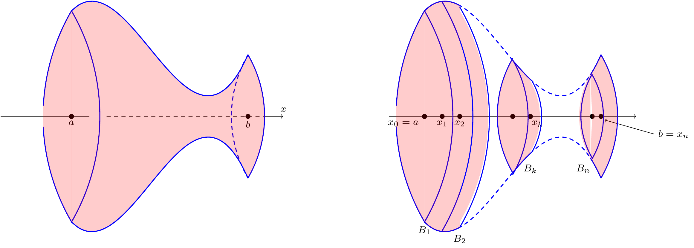
Figure 9.21: Splitting a volume into small cylinders

Namely: \[\text{vol}(R_C)=\sum_{k=1}^{n}\text{vol}(B_k).\] When we take the limit on the right hand side of the above equation we will get (9.4).

The volume is a particular example of a prism and its volume is the area of the base multiplied by the height:

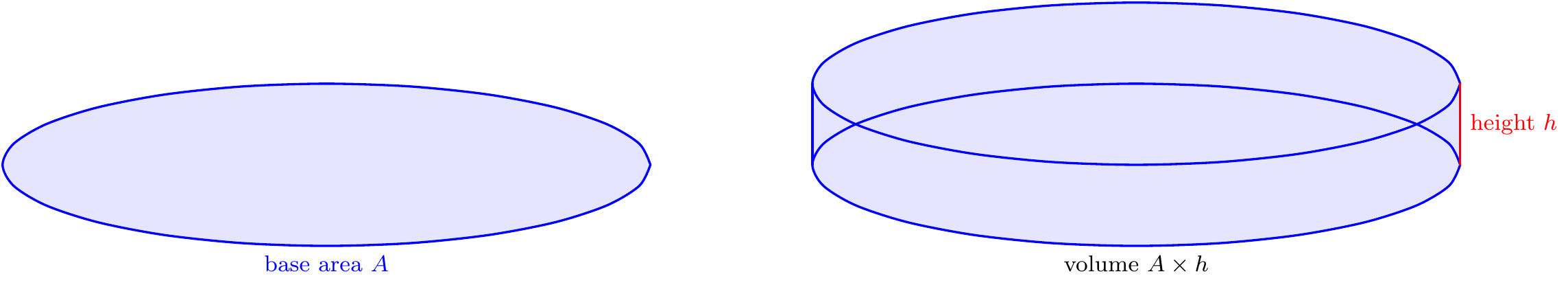
Figure 9.22: Volume of a cylinder

This is just a very flat cylinder, and we know that the volume of a cylinder of radius $r$ and height $h$ is just $\pi r^2h$.

We are taking a slice which has width $\delta x$ ($=x_{n+1}-x_n$), and we are going to imagine that $x_n$ and $x_{n+1}$ are sufficiently close that the function doesn’t change much between them. So the radius of the cylinder is $|f(x_n)|$. Substituting into the formula for the volume of the cylinder, we get \[\pi|f(x_n)|^2\delta x=\pi f(x_n)^2\delta x.\]

Therefore, we have justified the following theorem:

Theorem 9.6 If $f(x)$ is a continuous function on an interval $[a,b]$ then the volume of the solid $R_C$ obtained by rotating the region bounded between the $x$-axis and the curve $C=\{(x,f(x))\,|\,x\in[a,b]\}$ about the $x$-axis is given by \[\mathrm{vol}(R_C)=\pi\int_a^bf(x)^2~dx.\]

Example 9.13 As an application of the formula, we calculate the volume of the region bounded by the sphere of radius $R$. We know that the sphere of radius $R$ is obtained by rotating the graph of the function $f(x)=\sqrt{R^2-x^2}$ about the $x$-axis over the interval $[-R,R]$. So the volume of the ball of radius $R$ is \[\begin{aligned} \text{volume}(\text{ball of radius }R)&=\pi\int_{-R}^R\left(f(x)\right)^2~dx=\pi\int_{-R}^RR^2-x^2~dx=\pi\left[\left(R^2x-\frac{x^3}3\right)\right]_{-R}^R\\ &=\frac43\pi R^3.\end{aligned}\]

Example 9.14 Given the ellipse in the plane determined by the equation $\frac{x^2}{a^2}+\frac{y^2}{b^2}=1$, we can rotate the curve about the $x$-axis to obtain an ellipsoid. We can calculate the volume of the bounded solid using Theorem 9.6. To do this, we must first express $y$ in terms of $x$. \[\frac{x^2}{a^2}+\frac{y^2}{b^2}=1~\Leftrightarrow \frac{y^2}{b^2}=1-\frac{x^2}{a^2}=\frac{a^2-x^2}{a^2}~\Leftrightarrow~y^2=\frac{b^2(a^2-x^2)}{a^2}.\] To determine the region we are integrating over, we must solve for $y=0$; \[y=0~\Leftrightarrow~0=\frac{b^2(a^2-x^2)}{a^2}=\frac{b^2(a-x)(1+x)}{a^2},\] i.e., $y=0$ at $x=-a$ and $x=a$. Hence the volume of the ellipsoid is \[\pi\int_{x=-a}^{a}y^2~dx=\int_{-a}^{a}\frac{b^2(a^2-x^2)}{a^2}~dx=\frac{\pi b^2}{a^2}\int_{x=-a}^aa^2-x^2~dx=\frac{\pi b^2}{a^2}\frac43 a^3=\frac43\pi b^2a\] where the penultimate equality comes by replacing $R$ by $a$ in Example 9.13.

Example 9.15 To generalise the above example, we will now quickly calculate the volume bounded by a general ellipsoid given by the locus of $\frac{x^2}{a^2}+\frac{y^2}{b^2}+\frac{z^2}{c^2}=1$ using the linear algebra that we have learned. Note that the map \[L:\begin{pmatrix}x\\y\\z\end{pmatrix}\longmapsto \begin{pmatrix} a&0&0\\ 0&b&0\\ 0&0&c \end{pmatrix} \begin{pmatrix} x\\y\\z \end{pmatrix}= \begin{pmatrix} ax\\mathbf{y}\\cz \end{pmatrix},\] induces a bijection (exercise) from the unit ball $B$ to the region bounded by the ellipsoid $E$ \[L: B=\{(x,y,z\in\mathbb{R}^3~|~x^2+y^2+z^2\leq1\}~\longrightarrow~ E=\left\{(x,y,z)\in\mathbb{R}^3~\left|~\frac{x^2}{a^2}+\frac{y^2}{b^2}+\frac{z^2}{c^2}\leq 1 \right\}\right..\] Thus, \[\begin{equation} \mathrm{volume}(E)=\det\begin{pmatrix} a&0&0\\ 0&b&0\\ 0&0&c \end{pmatrix} \mathrm{volume}(B)=abc\times\mathrm{volume}(B)=\frac43\pi abc \tag{9.5} \end{equation}\] from Example 9.13.

We observe that the volume of the solid bounded by the ellipsoid in Example 9.14 is consistent with the general formula that we found in Example 9.15. When the ellipse in the plane determined by the equation $\frac{x^2}{a^2}+\frac{y^2}{b^2}=1$ is rotated 90 degrees onto the $yz$-plane, we note that the curve intersects the $z$-axis at $z=b$. Thus, the solid in Example 9.14 is the region given by the locus of \[\frac{x^2}{a^2}+\frac{y^2}{b^2}+\frac{z^2}{b^2}\leq1.\] Setting $c=b$ in (9.5) gives the result obtained in Example 9.14.

It is now time to start thinking about integrating functions of two variables over a region in the plane.