10 Integration of functions of two variables
Reflection on the definition of the definite integral of a function of one variable over a fixed domain leads to a natural generalisation of the definite integral of a function with more than \(n\) variables over a subset of \(\mathbb{R}^n\). In this chapter, we will see how the story unfolds when we restrict our attention to functions of two variables.
10.1 Double integrals
We have seen that integration of functions with a single variable is a versatile operation that allows us to calculate areas under the graphs of functions, arc lengths, as well as certain surface areas and volumes of regions in three space. In most cases however, regions in \(\mathbb{R}^3\) are not obtained by rotating a domain in a plane about an axis. For example, we currently do not know how to calculate the volume of any object without axial symmetry. In these next two sections we will learn how to calculate the volume under the graph of a function with two variables.
Very loosely, when we calculate the definite integral \(f:[a,b]\rightarrow\mathbb{R}\), we break the domain \([a,b]\) up into regions \(R_1,\dots,R_n\) (which are just intervals), choose a point \(x_1,\dots,x_n\) in each region and use the sum of the areas of the rectangles with base \(R_i\) and height \(f(x_i)\) to approximate the area under the graph. As we let the maximum length/diameter of the \(R_i\) go to zero, the number of regions increases, and we define \[\int_a^bf(x)\,dx=\lim_{\text{max length}(R_i)\to0}\sum_if(x_i)\,\text{length}(R_i)\] when the answer is independent of our choice of \(R_i\) and \(x_i\).
One dimension up, a “double integral” of a function \(f:\mathbb{R}^2\rightarrow\mathbb{R}\) will be defined as the limit of volumes of cuboids that approximate the volumes under the graph of \(f(x,y)\):
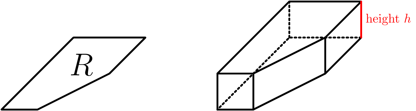
Figure 10.1: Volumes over regions
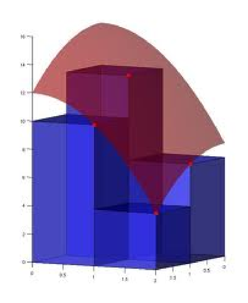
Figure 10.2: Approxmating volumes under surfaces with cuboids
We now use this interpretation to give a loose definition of the double integral of a function \(f:D\subseteq\mathbb{R}^2\rightarrow\mathbb{R}\).
Given a domain \(D\subseteq\mathbb{R}^2\), we can divide up the domain \(D\) up into disjoint regions \(R_1,\dots,R_n\) and choose points \((x_1,y_1),\dots,(x_n,y_n)\) in each region. We then “define” the double integral of \(f(x,y)\) over \(D\) to be \[\iint_Df(x,y)\,dA=\lim_{\text{max diameter}(R_i)\to0}\sum_if(x_i,y_i)\,\text{area}(R_i)\] when the answer is independent of our choice of \(R_i\) and \((x_i,y_i)\). The interpretation is that the sum on the right estimates the volume under the graph of a function, and in the limit we get the signed volume. We will call our loose definition the “Riemann sum” definition of the integral.
We should remark that \(\iint_Df(x,y)\,dA\) is one notation for this “double integral”; we will see others later. The “\(dA\)” refers to the fact that we are taking a limit of sums over little areas.
As with definite integrals of a function of a single variable, calculating a definite integral directly from the definition is not straightforward.
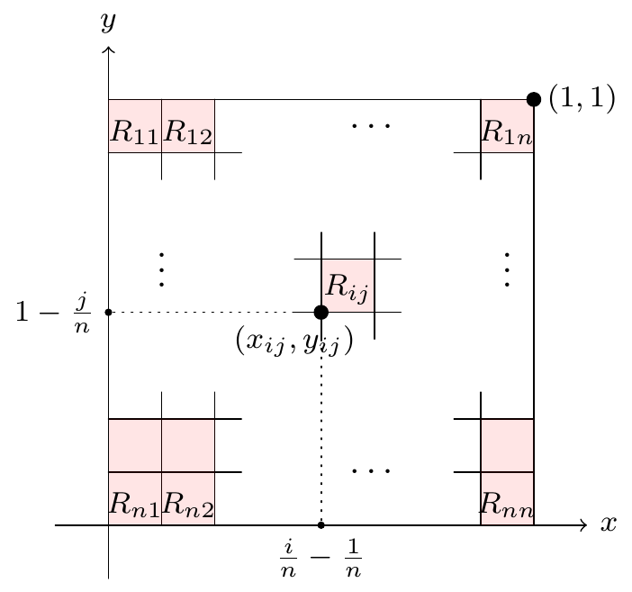
Figure 10.3: Spliting the square into small squares
The area of \(R_{ij}=\frac{1}{n^2}\) and \(\text{area}(R_i)\rightarrow0\) as \(n\rightarrow\infty\). So the double integral is given by \[\begin{aligned} \iint_S f(x,y)\,dA&=\lim_{\text{max diameter}(R_i)\rightarrow 0}\sum f(x_{ij},y_{ij})\text{area}(R_i)=\lim_{\text{max diameter}(R_i)\rightarrow 0} \sum x_{ij}y_{ij}\text{area}(R_i)\\ &=\lim_{\text{max diameter}(R_i)\rightarrow 0} \sum \left(\frac{i-1}n\right)\left(1-\frac jn\right)\frac{1}{n^2}=\lim_{n\rightarrow \infty} \sum_{j=1}^{n} \sum_{i=1}^n \left(\frac{i-1}n\right)\left(1-\frac jn\right)\frac{1}{n^2}\\ &=\lim_{n\rightarrow \infty} \sum_{i=1}^{n} \sum_{j=1}^n \frac{1}{n^4}(i-1)(n-j)=\lim_{n\rightarrow \infty} \frac{1}{n^4}\sum_{i=1}^{n} \sum_{j=1}^n (i-1)(n-j)\\ &=\lim_{n\rightarrow \infty} \frac{1}{n^4}\sum_{i=1}^{n} (i-1)\sum_{j=1}^n (n-j)=\lim_{n\rightarrow \infty} \frac{1}{n^4}\sum_{i=1}^{n} (i-1) \left((n-1)+(n-2)+\dots (n-n)\right)\\ &=\lim_{n\rightarrow \infty} \frac{1}{n^4}\sum_{i=1}^{n} (i-1) \Big(n\times n-(1+2+\dots n)\Big)\\ &=\lim_{n\rightarrow \infty} \frac{1}{n^4}\sum_{i=1}^{n} (i-1) \left(n^2-\frac{n(n-1)}2\right)=\lim_{n\rightarrow \infty} \frac{1}{n^4}\left(n^2-\frac{n(n-1)}2\right)\sum_{i=1}^{n} (i-1)\\ &=\lim_{n\rightarrow \infty} \frac{1}{n^4}\left(\frac{n^2+n}2\right)\Big((1-1)+(2-1)+\dots+(n-1)\Big)\\ &=\lim_{n\rightarrow \infty} \frac{1}{n^4}\left(\frac{n^2+n}2\right)\left((1+2+\dots + n)+n(-1)\right)\\ &=\lim_{n\rightarrow \infty} \frac{1}{n^4}\left(\frac{n^2+n}2\right)\left(\frac{n(n+1)}2-n\right)&=\lim_{n\rightarrow \infty} \frac{1}{n^4}\left(\frac{n^2+n}2\right)\left(\frac{n^2-n}2\right)\\ &=\frac{1}4 \lim_{n\rightarrow \infty} \frac{n^4-n^2}{n^4}=\frac{1}4 \lim_{n\rightarrow \infty} 1-\frac{1}{n^2}=\frac{1}4.\end{aligned}\]
Looking at the above example, it may not seem it, but integrating \(f(x,y)=xy\) over a square is a relatively simple special case where it is “easy” to use the definition of the integral to get an exact answer. In general, it is far from “easy” to calculate a double integral directly from the definition when the function or domain of integration are more complicated.
So we would like a more practical way to calculate double integrals. Fortunately, we will not have to get our hands dirty and work with the explicit “Riemann sum” definition of the double integral. As with integration for functions of a single variable, we will see that double integrals can be directly calculated if you know how to find the “antiderviative” of a function. In particular we will see that the following theorem is true (where, as usual, we won’t say precisely what “nice” means, but every function you are likely to work with in practice will be “nice”; see Example 10.6 to persuade yourself that the result isn’t true for any function at all!):

Figure 10.4: Diagram for the theorem
Then \[\iint_D f(x,y)\,dA=\int_{x=a}^{x=b}\left(\,\int_{y=g(x)}^{y=h(x)}f(x,y)\,dy\right)dx.\]
So if we can integrate a function with one variable then we can integrate a function with two variables! The integral on the right in Theorem 10.1 is called an “iterated” integral. We usually omit the brackets, and also the variables in the limits, and simply write \[\iint_D f(x,y)\,dA=\int_a^b\int_{g(x)}^{h(x)}f(x,y)\,dy\,dx.\] With an iterated integral like this, we start by evaluating the inner integral, \(\int_{g(x)}^{h(x)}f(x,y)\,dy\), which means that we regard \(x\) as constant, and integrate with respect to \(y\), with lower limit \(y=g(x)\) and upper limit \(y=h(x)\). This gives the area \(A_x\) under the curve \(f(x,y)\) – where we regard \(x\) as constant – between \(y=g(x)\) and \(y=h(x)\). We thicken this to get a slice between \(x\) and \(x+\delta x\), assuming that \(\delta x\) is so small that the function barely changes. Then the slice between \(x\) and \(x+\delta x\) will have volume approximately \(A_x\delta x\). Then we add these volumes up over all the slices to get the whole volume, which will be the integral \(\int_a^bA_x\,dx\).
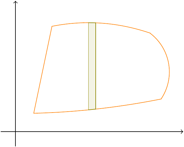
Figure 10.5: Splitting the region into strips
Note that the inner integral usually has limits which depend on \(x\), whereas the outer integral will have limits which don’t depend on any variables.
To illustrate how easy it can be to calculate an iterated integral, we will verify that the calculation of the double integral in the previous example agrees with what we get when we calculate the iterated integral.
Our only explicitly calculated iterated integral so far has been over a square. Let’s see an integral over a less simple domain.
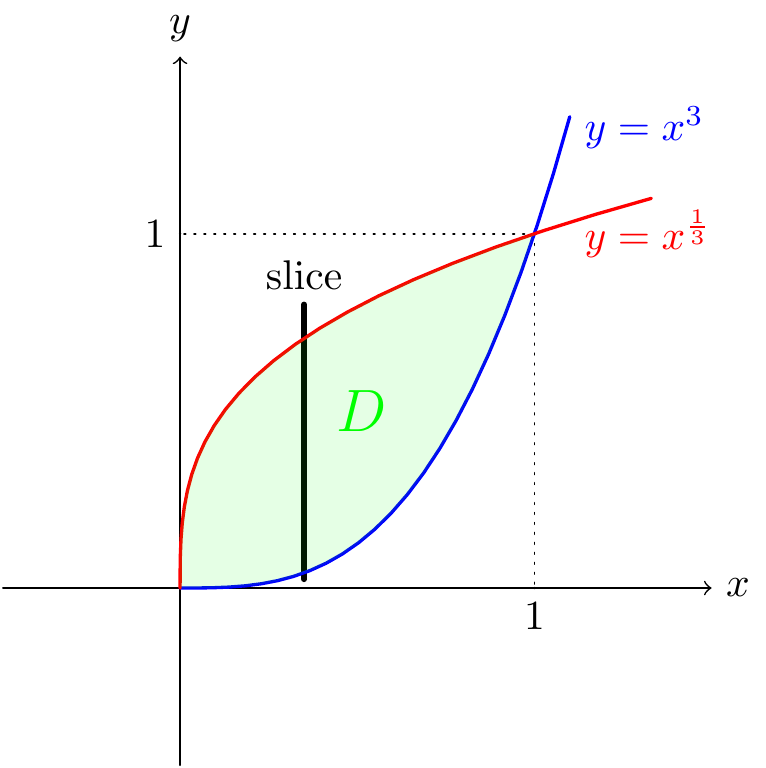
Figure 10.6: Vertical strips for the region in the example
We get \[\begin{aligned} \iint_D xy~dy\,dx&=\int_{x=0}^{x=1}\int_{y=x^3}^{y=x^{\frac{1}{3}}}xy~dy\,dx=\int_0^1\left[\frac{xy^2}{2}\right]_{y=x^3}^{y=x^{\frac{1}3}}~dx\\ &=\frac{1}2\int_0^1x^{\frac53}-x^7~dx=\frac{1}2\left[\frac38x^{\frac83}-\frac{1}8x^8\right]_{x=0}^{x=1}=\frac{1}8.\end{aligned}\]
Note that we have always been integrating first with respect to \(x\). Of course, we can relabel \(x\) and \(y\) (i.e., slice along sections parallel to the \(y\)-axis). This gives:
Theorem 10.2 If \(f(x,y)\) is a nice function defined on a domain \(D=\{(x,y):g(y)\le x\le h(y),\,a \le y\le b\}\), then \[\iint_D f(x,y)\,dA=\int_{y=a}^{y=b}\left(\,\int_{x=g(y)}^{x=h(y)}f(x,y)\,dx\right)dy.\]
Of course, we write \(\int_a^b\int_{g(y)}^{h(y)}f(x,y)\,dx\,dy\) for this, and we get the variables for the limits from the order in which the \(dx\) and \(dy\) appear.
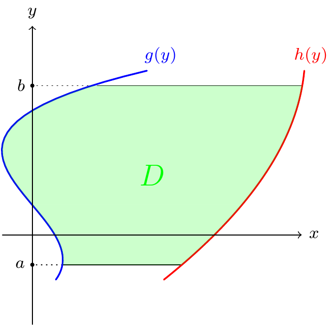
Figure 10.7: Integrating over horizontal strips
This ability to integrate first with respect to \(x\) of \(y\) might seem irrelevant, however there are cases where it can be very useful: sometimes the integral might be impossible with one variable taken first, but possible with the other.
Example 10.4 Note that we cannot integrate \(f(x,y)=ye^{-x^3}\) directly with respect to \(x\), so we cannot directly evaluate \[\int_{y=0}^{y=1}\int_{x=y}^{x=1} ye^{-x^3}~dx\,dy.\] However, we will see that the integral simplifies if we integrate the function \(f(x,y)\) first with respect to \(y\). To reverse the order of integration we must understand the domain \(T\) that we are integrating over.
For every \(y\in[0,1]\), when we slice parallel to the \(x\)-axis, the \(x\)-coordinate varies from \(y\) to \(1\). Varying \(y\) from 0 to 1, we see that \(T\) is the triangle with vertices \((0,0)\), \((1,0)\), \((1,1)\) (see the left hand picture below). So we are integrating over the domain \(T=\{(x,y)~|~0\le x\le y\le1\}\).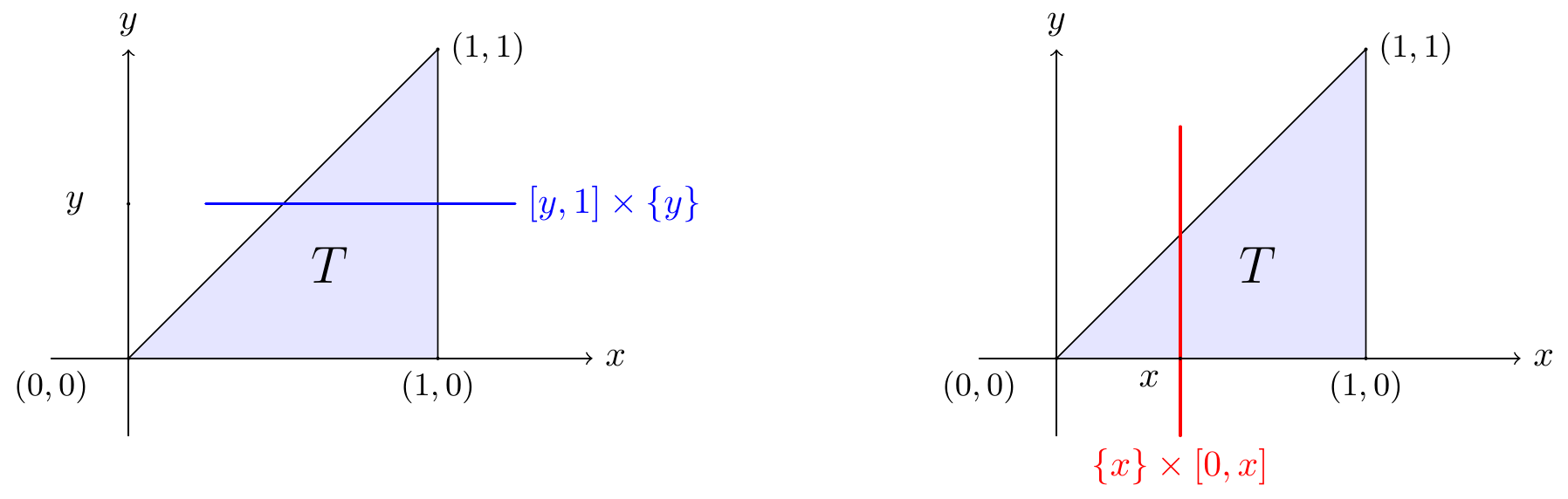
Figure 10.8: Horizontal and vertical strips
If we integrate first with respect to \(y\) then we fix \(x\) and \(y\) varies from \(0\) to \(x\) (see the right hand side of the picture). Hence \[\begin{aligned} \int_{y=0}^{y=1}\int_{x=y}^{x=1} ye^{-x^3}~dx\,dy&=\iint_Tye^{-x^3}~dy\,dx=\int_{x=0}^{x=1}\int_{y=0}^{y=x}ye^{-x^3}~dy\,dx\\ &=\int_{x=0}^{x=1}\left[\frac{y^2}2e^{-x^3}\right]_{y=0}^{y=x}~dx=\frac{1}2\int_{x=0}^{x=1}x^2e^{-x^3}~dx\\ &=\frac{1}2\left(-\frac{1}3e^{-x^3}\right)_{x=0}^{x=1}=\frac{1-e^{-1}}6.\end{aligned}\]
By carefully considering the “Riemann sum” definition above, or by thinking about the geometric interpretation, we can see that the double integral has the following useful properties:
- Domain area
The area of a domain is equal to the volume of a prism of height one over that domain: \[\iint_D1~dA=\text{area}(D).\]
- Linearity
the sum of volumes is a sum of volumes; given \(f,g:\mathbb{R}^2\rightarrow\mathbb{R}\), \[\iint_Df(x,y)+g(x,y)~dA=\iint_Df(x,y)~dA+\iint_Dg(x,y)~dA.\]
- Scaling
scaling the height of an object scales the volume by the same amount; given \(a\in\mathbb{R}\) and \(f:\mathbb{R}^2\rightarrow\mathbb{R}\), \[\iint_Daf(x,y)~dA=a\iint_Df(x,y)~dA.\]
- Domain additivity
The volume of two disjoint objects is the sum of the volumes of the individual pieces; given a disjoint union \(D=D_1\cup D_2\) \[\iint_Df(x,y)~dA=\iint_{D_1}f(x,y)~dA+\iint_{D_2}f(x,y)~dA.\]
These observations are elementary but can be useful.
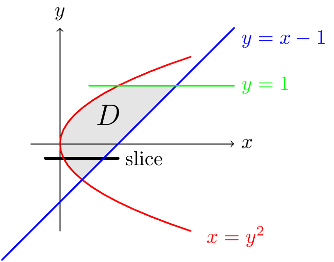
Figure 10.9: Finding an area by double integration
We know that \[\text{area}(D)=\iint_D~dA.\] Over \(D\), the value of \(x\) varies from \(y^2\) to \(y+1\), and the value of \(y\) varies from the \(y\) coordinate of the intersection between \(y=x-1\) and \(y=-\sqrt x\) to the \(y=1\). Now \(y=x-1\) and \(x=y^2\) if and only if \[-\sqrt y=y^2-1~\Longrightarrow~y^2-y-1=0 \Longrightarrow~y=\frac{1\pm\sqrt5}2.\] From the picture, we see that \(y\) varies from \(\frac{1-\sqrt5}2\). That is, \[D=\left\{(x,y)~|~y^2\le x\le y+1,\tfrac{1-\sqrt5}2\le y\le1\right\}.\] Hence \[\begin{aligned} \text{area}(D)&=\iint_D~dA=\int_{y=\frac{1-\sqrt5}{2}}^1\int_{x=y^2}^{x=y+1}~dx\,dy=\int_{y=\frac{1-\sqrt5}{2}}^1\left[x\right]_{x=y^2}^{x=y+1}~dy=\int_{y=\frac{1-\sqrt5}{2}}^1y+1-y^2~dy\\ &=\left[\frac{y^2}{2}+y-\frac{y^3}{3}\right]_{y=\frac{1-\sqrt5}{2}}^1=\frac{7}{6}-\frac{1}{3}\left(\frac{6-2\sqrt5}{4}+\frac{1-\sqrt5}{2}-\frac{16-8\sqrt5}{8}\right)\\ &=\frac{7+4\sqrt5}{6}.\end{aligned}\]
Example 10.6 Again, however, I feel morally obliged to point out that switching the order of the variables invovled in a double integral isn’t actually always valid. As usual, it depends on the fact that the function \(f\) being integrated is somehow “nice”. This will be the case for all functions you ever meet in practice; if you can write down a function with a nice expression, it is almost certain that it will be “nice”, and that it is absolutely fine to switch the variables. But here’s a function \(f\) where it isn’t true that \[\int_0^1\int_0^1f(x,y)~dx\,dy=\int_0^1\int_0^1f(x,y)~dy\,dx.\] Indeed, let’s consider \[f(x)=\left\{ \begin{array}{ll} 1/y^2,&\mbox{for $0<x<y<1$},\\ -1/x^2,&\mbox{for $0<y<x<1$},\\ 0,&\mbox{otherwise}. \end{array} \right.\] For \(0<y<1\), we have \[\int_0^1f(x,y)~dx=\int_0^y\frac{dx}{y^2}-\int_y^1\frac{dx}{x^2}=\left[\frac{x}{y^2}\right]_{x=0}^{x=y}-\left[-\frac{1}{x}\right]_{x=y}^{x=1}=\frac{1}{y}+\frac{(1-y)}{y}=1.\] So \[\int_0^1\int_0^1f(x,y)~dx\,dy=\int_0^11~dy=1.\]
Similarly, for \(0<x<1\), we have \[\int_0^1f(x,y)~dy=-\int_0^x\frac{dy}{x^2}+\int_x^1\frac{dy}{y^2}=-\frac{1}{x}-\frac{(1-x)}{x}=-1,\] and \[\int_0^1\int_0^1f(x,y)~dy\,dx=\int_0^1-1~dy=-1.\]10.2 Change of variable
It is a direct consequence of the Fundamental Theorem of Calculus that when we change variables with a map \(x\mapsto u(x)\) we get \[\int_a^bf(u(x))\frac{du}{dx}~dx=\int_{u(a)}^{u(b)}f(u)~du.\] Similarly, when we take \(x\mapsto x(u)\) we get \[\int_{a}^{b}f(x)~dx=\int_{x^{-1}(a)}^{x^{-1}(b)}f(x(u))\frac{dx}{du}~du.\] In the first case, we have seen a geometric justification of the substitution rule. The substitution \(x\mapsto u(x)\) does not affect the height of the function but “stretches” the base domain. So the base lengths \(\delta x\) of rectangles that approximate the area under the graph are changed to \(\delta u\approx\frac{du}{dx}\delta x\). Taking limits, we get the stated substitution rule.
When we work with double integrals, changing variables corresponds to transforming a domain in the \(uv\)-plane to a domain in the \(xy\)-plane. So, we have a map \[T:S_{uv}\subseteq \mathbb{R}^2\rightarrow C_{xy}\subseteq\mathbb{R}^2, \text{ defined by }(u,v)~\mapsto~(x(u,v),y(u,v)).\] We will see that when \(T\) is bijective that the change of variables corresponds to the following integral identity \[\iint_{C_{xy}}f(x,y)~dx\,dy=\iint_{S_{uv}}f(x(u,v),y(u,v))\left|\frac{\partial(x,y)}{\partial(u,v)}\right|~du\,dv.\] where \[\frac{\partial(x,y)}{\partial(u,v)}=\begin{vmatrix} \frac{\partial x}{\partial u}&\frac{\partial x}{\partial v}\\ \frac{\partial y}{\partial u}&\frac{\partial y}{\partial v} \end{vmatrix}=\frac{\partial x}{\partial u}.\frac{\partial y}{\partial v}- \frac{\partial x}{\partial v}.\frac{\partial y}{\partial u}.\]
As a special case we start by considering what happens when \(T\) is multiplication by a \(2\times2\) matrix; if \(T:S_{uv}\rightarrow C_{xy}\) is a bijective map defined by \[\mathbf{u}=\begin{pmatrix}u\\v\end{pmatrix}\mapsto\begin{pmatrix}x(u,v)\\y(u,v)\end{pmatrix}=\begin{pmatrix}a&b\\c&d\end{pmatrix}\begin{pmatrix}u\\v\end{pmatrix}=\begin{pmatrix}au+bv\\cu+dv\end{pmatrix}\] then we know that \[\text{area}(C_{xy})=|\det A|.\text{area}(S_{uv})=|ad-bc|.\text{area}(S_{uv})=|x_uy_v-x_vy_u|.\text{area}(S_{uv})\] and with some careful thought, the claimed substitution rule for double integrals holds.
In general however, transforms of the plane are not obtained by multiplying by a matrix. The picture below shows the result of a very useful transform which is not obtained by multiplying by a matrix (why is this transform not obtained by matrix multiplication?).
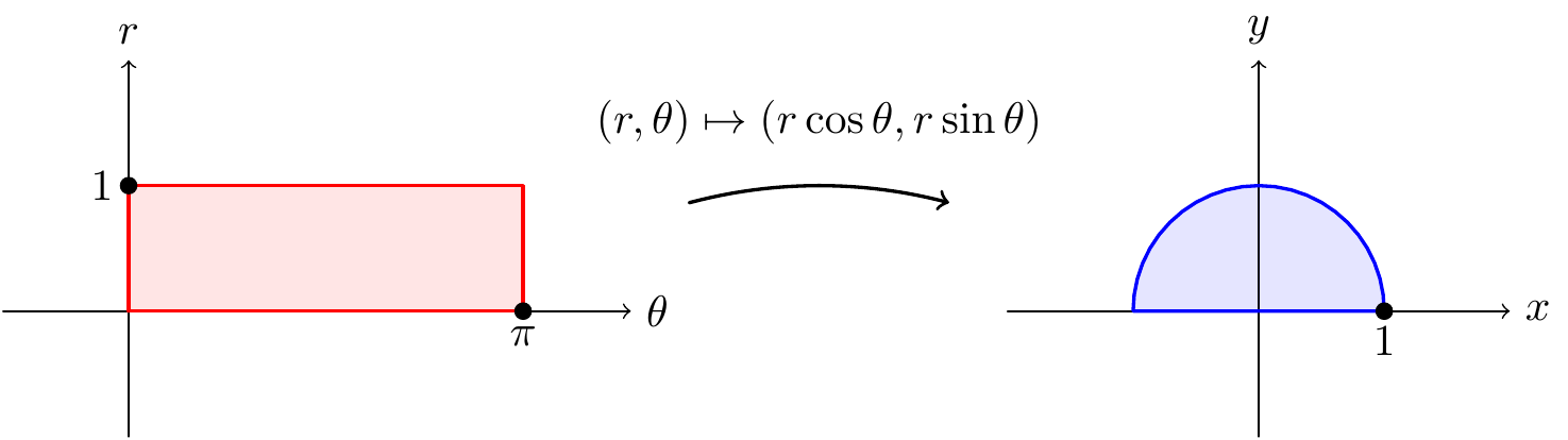
Figure 10.10: Rectangulars to polars
For a general mapping \(T:(u,v)\mapsto (x(u,v),y(u,v))\), with \(x(u,v)\) and \(y(u,v)\) differentiable, we have already seen using the Chain Rule that \[\delta x~\approx~ \frac {\partial x}{\partial u}\delta u+\frac {\partial x}{\partial v}\delta v,\qquad\delta y~\approx~ \frac {\partial y}{\partial u}\delta u+\frac {\partial y}{\partial v}\delta v\] i.e., \[\begin{pmatrix}\delta x\\\delta y\end{pmatrix}=\begin{pmatrix}\frac{\partial x}{\partial u} & \frac {\partial x}{\partial v}\\\frac {\partial y}{\partial u} & \frac {\partial y}{\partial v}\end{pmatrix}\begin{pmatrix}\delta u\\\delta v\end{pmatrix}.\] So, when distances are on a very small level, \(T\) behaves like multiplication by the matrix of first order derivatives shown above! We give this matrix of first order derivatives a name:
Definition 10.1 Given a transformation \(T:\mathbb{R}^2\rightarrow\mathbb{R}^2\) given by \((u,v)\mapsto (x(u,v),y(u,v))\), where \(x,y:\mathbb{R}^2\rightarrow\mathbb{R}\), we call \[J(T)=\begin{pmatrix}\frac{\partial x}{\partial u}&\frac{\partial x}{\partial v}\\\frac{\partial y}{\partial u}&\frac{\partial y}{\partial v}\end{pmatrix}\] the Jacobian matrix of \(T\). We call \(\det J(T)\) the Jacobian of the transformation and denote it by \(\frac{\partial(x,y)}{\partial(u,v)}\).
We have already indicated that the Jacobian measures the change of volume. The result is:
Theorem 10.3 (Change of variables) Let \(f(x,y)\) be an integrable function on \(D\subset\mathbb{R}^2\). If \(T:(u,v)\mapsto (x(u,v),y(u,v))\) is a bijective map from a domain \(T^{-1}(D)\) in the \(uv\)-plane to a domain \(D\) in the \(xy\)-plane with continuous partial derivatives \(\frac{\partial x}{\partial u}\), \(\frac{\partial x}{\partial v}\), \(\frac{\partial y}{\partial u}\) and \(\frac{\partial y}{\partial v}\), then \[\iint_Df(x,y)~dx\,dy=\iint_{T^{-1}(D)}f(x(u,v),y(u,v))\left|\frac{\partial(x,y)}{\partial(u,v)}\right|~du\,dv.\]
We now see how changing variables can simplify integrals in practice. Let us use this to evaluate the volume of a hemisphere:
Note that the calculation of the Jacobian in the previous example gives us:
We already noted this in Chapter 6, but it is so important that it does no harm to do it again!
We have already seen that iterated integrals can be used to calculate areas in the plane (see Example 10.5. Changing variables with iterated integrals can also help us calculate areas of particular types of domain in the plane.
Examples 10.7 and 10.8 evaluate double integrals by changing to polar coordinates. However, Theorem 10.4 is just a special case of Theorem 10.3, and changing to other coordinate systems can be useful when we calculate double integrals.
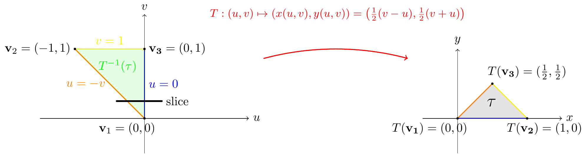
Figure 10.11: Change of variables for the example
We will now use Theorem 10.3 which states that \[\iint_{\tau}f(x,y)~dA=\iint_{T^{-1}(\tau)}f\Big(x(u,v),y(u,v)\Big)\left|\frac{\partial(x,y)}{\partial(u,v)}\right|~du\,dv.\]
When we change variables, if we integrate first with respect to \(u\) then \(u\) varies from \(u=-v\) to \(u=0\), as \(v\) varies from \(0\) to \(1\). We can easily calculate the Jacobian of our transform: \[J(T)=\begin{pmatrix}\frac{\partial x}{\partial u}&\frac{\partial x}{\partial v}\\\frac{\partial y}{\partial u}&\frac{\partial y}{\partial v}\end{pmatrix}=\begin{pmatrix}-\frac{1}2 & \frac{1}2 \\\frac{1}2 & \frac{1}2\end{pmatrix},\] and so \(\frac{\partial(x,y)}{\partial(u,v)}=-\frac{1}2\). Thus \[\begin{aligned} \iint_{\tau}f(x,y)~dA&=\int_{v=0}^{v=1}\int_{u=-v}^{u=0}\frac{1}2 e^{\frac uv}~du\,dv=\frac{1}2\int_{v=0}^{v=1}\left[ve^{\frac uv}\right]_{u=-v}^{u=0}~dv=\frac{1}2\int_{v=0}^{v=1}v(1-e^{-1})~dv\\ &=\frac{1}2\left[(1-e^{-1})\frac{v^{2}}2\right]_{v=0}^{v=1}=\frac{1-e^{-1}}4.\end{aligned}\]
As a second example of using double integration to calculate areas (see Example 10.5, we make use of the following fact (this was Corollary 6.1:
Theorem 10.5 If \(T:D\subseteq\mathbb{R}^2\rightarrow S\subseteq\mathbb{R}^2\) is a bijective transformation with \[(u,v)~\mapsto~(x(u,v),y(u,v))\] and inverse transformation \[(x,y)~\mapsto~(u(x,y),v(x,y))\] then \[\frac{\partial(x,y)}{\partial(u,v)}\times \frac{\partial(u,v)}{\partial(x,y)}=1.\]
The above theorem may seem technical, but it is basically a higher dimensional version of the chain rule \(\frac{dy}{dx}\frac{dx}{dy}=1\).
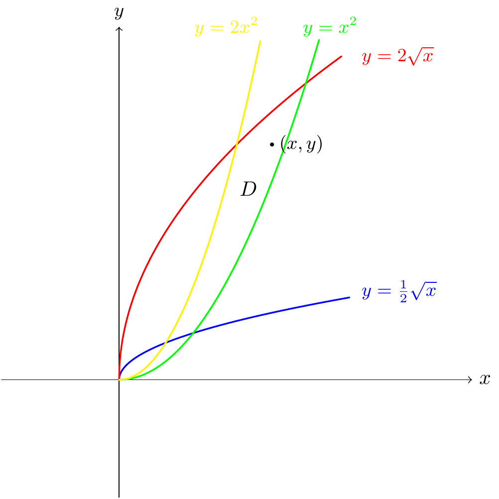
Figure 10.12: Change of variables for the example
If \((x,y)\in D\) then, by considering the position of the point relative to the curves that bound \(D\), we see that \[x^2\leq y\leq 2x^2,\qquad\frac{1}2\sqrt{x}\leq y\leq 2\sqrt{x}.\] When we divide both inequalities by \(y\) (which is positive) we get: \[\frac{1}2\le\frac{x^2}y\le1,\qquad\frac{1}2\leq \frac{\sqrt x}y\le2.\] We will calculate the area of \(D\) by considering the substitution \[u(x,y)=\frac{x^2}y,\qquad v(x,y)=\frac{\sqrt{x}}y.\] In this case, \[\frac{\partial(u,v)}{\partial(x,y)}=\begin{vmatrix}\frac{\partial u}{\partial x}&\frac{\partial v}{\partial x}\\\frac{\partial u}{\partial y}&\frac{\partial v}{\partial y}\end{vmatrix}=\begin{vmatrix}\frac{2x}y&-\frac{x^2}{y^2}\\\frac{1}{2y\sqrt x}&-\frac{\sqrt x}{y^2}\end{vmatrix}=-2\frac{x^{\frac32}}{y^3}+\frac{1}2\frac{x^{\frac32}}{y^3}=-\frac32\frac{x^{\frac32}}{y^3}=-\frac32v^3,\] so that \[\left|\frac{\partial(x,y)}{\partial(u,v)}\right|=\frac23v^{-3}\] by Theorem 10.5, and because \(v\) is positive. So the map \[T:R=\{(u,v)~|~\tfrac12\le u\le1,~\tfrac12\le v\le2\}~\rightarrow D\] is bijective (we first expressed the map in terms of \(T^{-1}\)) with Jacobian \(\frac23v^{-3}\). Hence \[\begin{aligned} \text{area}(D)&=\iint_D~dA=\iint_R\left|\frac{\partial(x,y)}{\partial(u,v)}\right|~du\,dv=\int_{v=\frac{1}2}^{v=2}\int_{u=\frac{1}2}^{u=1}\frac23v^{-3}~du\,dv\\ &=\int_{v=\frac{1}2}^{v=2}\left[\frac23v^{-3}u\right]_{u=\frac{1}2}^{u=1}~dv=\frac{1}3\int_{v=\frac{1}2}^{v=2}v^{-3}~dv\\ &=\left[-\frac{1}6v^{-2}\right]_{v=\frac{1}2}^{v=2}=\frac58.\end{aligned}\]
10.3 The Fundamental Theorem of Algebra
The Fundamental Theorem of Algebra states that the complex numbers \(\mathbb{C}\) are algebraically closed. This means that every non-constant polynomial with complex coefficients has a complex root.
Let’s give a proof of this, using multivariable calculus. In fact, this proof is (one of) Gauss’s original proofs, from 1816. Note that it doesn’t happen for the rationals \(\mathbb{Q}\) (think of \(x^2-2\)) or the reals \(\mathbb{R}\) (think of \(x^2+1\)). So this is a very special property of the complex numbers.
We are going to prove that if \[f(z)=z^d+a_{d-1}z^{d-1}+\cdots+a_1z+a_0\] is a polynomial of degree \(d\) with no complex roots, then \(d=0\). You should be able to convince yourself that this is exactly what we need.
Let’s write \(z=re^{i\theta}=r(\cos\theta+i\sin\theta)\). Then \(z^k=r^ke^{ik\theta}=r^k(\cos(k\theta)+i\sin(k\theta))\). Write \(f(z)=P(r,\theta)+iQ(r,\theta)\), so that \(P\) and \(Q\) are the real and imaginary parts of \(f\). Let’s also put \(a_k=b_k+ic_k\). Since \[f(z)=r^d(\cos(d\theta)+i\sin(d\theta))+(b_{d-1}+ic_{d-1})r^{d-1}(\cos(d-1)\theta+i\sin((d-1)\theta))+\cdots+(b_0+ic_0),\] we have: \[\begin{eqnarray*} P(r,\theta)&=&r^d\cos(d\theta)+b_{d-1}r^{d-1}\cos((d-1)\theta)-c_{d-1}r^{d-1}\sin((d-1)\theta)+\cdots+b_0,\\ Q(r,\theta)&=&r^d\sin(d\theta)+b_{d-1}r^{d-1}\sin((d-1)\theta)+c_{d-1}r^{d-1}\cos((d-1)\theta)+\cdots+c_0.\end{eqnarray*}\] Notice that:
\(\frac{\partial P}{\partial\theta}\) and \(\frac{\partial Q}{\partial\theta}\) vanish at \(r=0\), since the constant terms of \(P\) and \(Q\) don’t depend on \(\theta\);
\(P\), \(Q\), \(\frac{\partial P}{\partial r}\) and \(\frac{\partial Q}{\partial r}\) are all unchanged if \(\theta\) is changed into \(\theta+2\pi\) (we say that they are \(2\pi\)-periodic).
We are assuming that \(f\) has no complex roots, so \(P\) and \(Q\) do not simultaneously vanish, and so \(P^2+Q^2\) is never \(0\). Let’s put \[\begin{eqnarray*} U&=&\frac{PQ_r-QP_r}{P^2+Q^2}\\ V&=&\frac{PQ_\theta-QP_\theta}{P^2+Q^2}. \end{eqnarray*}\] (these are essentially the partial derivatives of \(\arctan(Q/P)\)).
You can check that \[\frac{\partial U}{\partial\theta}=\frac{\partial V}{\partial r}.\] Now notice that, as \(U\) is \(2\pi\)-periodic, \[\int_0^{2\pi}\frac{\partial V}{\partial r}\,d\theta=\int_0^{2\pi}\frac{\partial U}{\partial\theta}\,d\theta=[U]_{\theta=0}^{\theta=2\pi}=0.\] Therefore for any \(R>0\), \[\int_0^R\left(\int_0^{2\pi}\frac{\partial V}{\partial r}\,d\theta\right)\,dr=0.\] Exchanging the order of integration, we see that \[\int_0^{2\pi}\left(\int_0^R\frac{\partial V}{\partial r}\,dr\right)\,d\theta=0.\] We have that \[\int_0^R\frac{\partial V}{\partial r}\,dr=[V]_{r=0}^{r=R}.\] Now \(V\) vanishes when \(r=0\), since \(V=\dfrac{PQ_\theta-QP_\theta}{P^2+Q^2}\), and \(P_\theta\) and \(Q_\theta\) both vanish when \(r=0\), as already noted above. So \(\int_0^R\frac{\partial V}{\partial r}\,dr\) is simply the value of \(V\) at \(r=R\). But let’s work this out explicitly. From the formulae above for \(P\) and \(Q\), we have \[P_\theta=-dr^d\sin(d\theta)+\cdots,\qquad Q_\theta=dr^d\cos(d\theta),\] and \[\begin{eqnarray*} PQ_\theta-QP_\theta&=&(r^d\cos(d\theta)+\cdots)(dr^d\cos(d\theta)+\cdots)-(r^d\sin(d\theta)+\cdots)(-dr^d\sin(d\theta)+\cdots)\\ &=&(dr^{2d}\cos^2(d\theta)+\cdots)+(dr^{2d}\sin^2(d\theta)+\cdots)\\ &=&dr^{2d}+\cdots. \end{eqnarray*}\] And \[P^2+Q^2=(r^{2d}\cos^2(d\theta)+\cdots)+(r^{2d}\sin^2(d\theta)+\cdots)=r^{2d}+\cdots.\] So \[V=\frac{PQ_\theta-QP_\theta}{P^2+Q^2}=\frac{dr^{2d}+\cdots}{r^{2d}+\cdots}.\] Notice that as \(r\to\infty\), this approaches \(d\). Then \[\int_0^{2\pi}\left(\int_0^R\frac{\partial V}{\partial r}\,dr\right)\,d\theta=\int_0^{2\pi}V(R)\,d\theta\to\int_0^{2\pi}d\,d\theta=2\pi d.\] But we have already explained that this integral vanishes. It follows that \(d=0\).
10.4 Two beautiful corollaries
We’ll end our discussion in this chapter with two important results which can be derived from the theory of double integrals. You will have seen both before, but probably not their proofs.
10.4.1 \(\sum_{n=1}^\infty\frac{1}{n^2}\)
You may already have seen the statement of the theorem below. If so, you were probably struck by the appearance of \(\pi\), and wondered why the sum in the theorem should have anything to do with \(\pi\)!
We’ll give a proof using change of variables in a double integral. The result is due to Euler, although this proof isn’t the one he came up with (and there are many other proofs in addition).
Proof. Consider \(I=\int_0^1\int_0^1\frac{dx\,dy}{1-x^2y^2}\). We will evaluate it in two ways.
Firstly, we use the identity \[\frac{1}{1-t}=1+t+t^2+\cdots,\] and write the integral as \[\int_0^1\int_0^11+x^2y^2+x^4y^4+x^6y^6+\cdots\,dx\,dy,\] and notice that \(\int_0^1\int_0^1x^ky^k\,dx\,dy=\frac{1}{(k+1)^2}\). So one way to evaluate the integral gives \[1+\frac{1}{3^2}+\frac{1}{5^2}+\frac{1}{7^2}+\cdots.\]
But it turns out that we can find a substitution which allows us to compute the integral exactly. Put \[x=\frac{\sin u}{\cos v},\qquad y=\frac{\sin v}{\cos u}.\] The Jacobian of this is: \[\begin{aligned} \left|\frac{\partial(x,y)}{\partial(u,v)}\right|&=\begin{vmatrix}\cos u/\cos v&\sin u\sin v/\cos^2v\\\sin u\sin v/\cos^2u&\cos v/\cos u\end{vmatrix}\\ &=1-\frac{\sin^2u\sin^2v}{\cos^2u\cos^2v}\\ &=1-x^2y^2.\end{aligned}\] We need to see what the region \(\{(x,y)~|~0\le x\le1,~0\le y\le1\}\) maps to in terms of \(u\) and \(v\). Notice that if \(x>0\) and \(y>0\), then we can take \(0<u<\pi/2\) and \(0<v<\pi/2\). Now, if \(x\le1\), this means that \(\sin u\le\cos v\). But \(\cos v=\sin(\pi/2-v)\), so we need \(\sin u\le\sin(\pi/2-v)\). Since the graph of \(\sin\) is increasing, this must mean that \(u\le\pi/2-v\), so that \(u+v\le\pi/2\). It is easy to see that the same result (with the same argument) comes from the inequality \(y\le1\). So the square region we started with in the \((x,y)\)-plane maps to the region \(A=\{(u,v)~|~u>0,~v>0,~u+v<\pi/2\}\), which is a triangle of area \(\pi^2/8\).
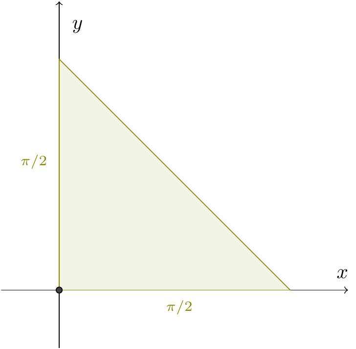
Figure 10.13: The triangle in the theorem
By substituting, we see that \[\int_0^1\int_0^1\frac{dx\,dy}{1-x^2y^2}=\iint_A1\,du\,dv=\frac{\pi^2}{8}.\]
Now we see that \[1+\frac{1}{3^2}+\frac{1}{5^2}+\frac{1}{7^2}+\cdots=\frac{\pi^2}{8}.\] Notice that this left-hand side is equal to \[\begin{eqnarray*} &&\left(1+\frac{1}{2^2}+\frac{1}{3^2}+\frac{1}{4^2}+\cdots\right)-\left(\frac{1}{2^2}+\frac{1}{4^2}+\frac{1}{6^2}+\frac{1}{8^2}+\cdots\right)\\ &=&\left(1+\frac{1}{2^2}+\frac{1}{3^2}+\frac{1}{4^2}+\cdots\right)-\frac{1}{4}\left(1+\frac{1}{2^2}+\frac{1}{3^2}+\frac{1}{4^2}+\cdots\right)\\ &=&\frac{3}{4}\left(1+\frac{1}{2^2}+\frac{1}{3^2}+\frac{1}{4^2}+\cdots\right). \end{eqnarray*}\] So \[\frac{3}{4}\left(1+\frac{1}{2^2}+\frac{1}{3^2}+\frac{1}{4^2}+\cdots\right)=\frac{\pi^2}{8},\] and we deduce that \[1+\frac{1}{2^2}+\frac{1}{3^2}+\frac{1}{4^2}+\cdots=\frac{\pi^2}{6},\] as claimed. ```
10.4.2 The Gaussian integral
It could be argued that the Gaussian integral \[I=\int_{-\infty}^{\infty}e^{-x^2}~dx\] is the most important integral for humanity to evaluate. The Central Limit Theorem tells us that averages of samples are distributed like the curve \(f(x)=e^{-x^2}\); all social and physical sciences use this mathematical fact and so the modern world depends us being able to normalise \(f(x)=e^{-x^2}\) (i.e., divide \(f(x)\) by \(I\))!
We will use double integration to calculate \(I\). To do this, we will use the following simple observation: since \(g(y)\) is treated as a constant when we integrate with respect to \(x\), we have the following identity \[\int_{y=a}^{y=b}\int_{x=c}^{x=d}f(x)g(y)~dx\,dy=\left(\int_{a}^{b}g(y)~dy\right)\left(\int_{c}^{d}f(x)~dx\right).\]