3 Matrices

3.1 Basic definition

We’ve already seen that a matrix is just an array of numbers, put inside brackets.

Definition 3.1

1. An \(m\times n\) matrix is an array of numbers: \[\begin{pmatrix}a_{11}&\ldots&a_{1n}\\\vdots&\ddots&\vdots\\a_{m1}&\ldots&a_{mn}\end{pmatrix}\] with \(m\) rows and \(n\) columns.

2. If \(m=n\), \(A\) is a square matrix.

3. The collection of all \(m\times n\) matrices is denoted \(M_{m,n}(\mathbb{R})\); if \(m=n\), we usually just write \(M_n(\mathbb{R})\) for the square \(n\times n\) matrices.

4. The zero \(m\times n\) matrix is the \(m\times n\) matrix with all entries equal to \(0\).

5. A column vector is a matrix with 1 column (so an \(m\times1\) matrix) and a row vector is a matrix with 1 row (a \(1\times n\) matrix). The collection of column vectors with \(m\) entries is denoted \(\mathbb{R}^m\), and you should already be familiar with \(\mathbb{R}^2\) and \(\mathbb{R}^3\) from school; we just get the usual vectors in 2 or 3 dimensional space. Column vectors in \(\mathbb{R}^n\) are often written in bold type, e.g., \(\mathbf{v}\), but equally often this doesn’t happen, and the meaning is left to the context. I’ll try to write them in bold type.

6. The entry \(a_{ij}\) is the \(ij\)th element.

7. The leading diagonal of a square matrix is the collection of entries \(a_{11}\), \(a_{22}\),….

8. The trace of a square matrix is the sum of the entries on the leading diagonal.

9. A diagonal matrix is a square matrix whose only non-zero entries are on the leading diagonal.

10. The identity matrix is the diagonal square matrix with \(1\)s on the leading diagonal. The reason for the terminology will be clear later.

11. Two matrices \(A\) and \(B\) are equal if they are both \(m\times n\) matrices for some \(m\) and \(n\), and if \(a_{ij}=b_{ij}\) for all \(i=1,2,\ldots,m\) and \(j=1,2,\ldots,n\).

12. The transpose \(A^T\) of the matrix \(A\) is the matrix with rows and columns interchanged. (So if \(A\) is an \(m\times n\) matrix, its transpose is an \(n\times m\) matrix.)

13. A matrix is symmetric if \(A^T=A\), and antisymmetric if \(A^T=-A\).

\[\begin{pmatrix}2&1\\3&4\end{pmatrix}~(2\times 2),\quad\begin{pmatrix}1&7&3\\2&4&1\\8&2&3\end{pmatrix}~(3\times 3)\] are square matrices, and \[\begin{pmatrix}2&1&7\\1&4&2\end{pmatrix}~(2\times 3),\quad\begin{pmatrix}1&2\\1&3\\3&7\end{pmatrix}~(3\times 2)\] are not.

3.2 Basic properties

3.2.1 Matrix addition

Two matrices \(A\) and \(B\) can only be added if they have the same size. If \(A\) and \(B\) are \(m\times n\)-matrices then \(C=A+B\) is an \(m\times n\)-matrix with elements \[c_{ij}=a_{ij}+b_{ij}\quad(i=1,2,\ldots,m,~j=1,2,\ldots,n).\] For example, if \[A=\begin{pmatrix} 1&3&1\\ 2&7&-2 \end{pmatrix},\qquad B=\begin{pmatrix} -2&1&4\\ -3&1&2 \end{pmatrix},\] then \[C=A+B=\begin{pmatrix} -1&4&5\\ -1&8&0 \end{pmatrix}.\]

Let’s just stress the main requirement:

Two matrices \(A\) and \(B\) can be added only when they have exactly the same number of rows and the same number of columns.

For any two matrices \(A\) and \(B\) of the same size, matrix addition is commutative: \(A+B=B+A\).

For any 3 matrices \(A,B\) and \(C\) of same size addition is associative \[(A+B)+C=A+(B+C),\] and we often simply write \(A+B+C\) for the answer.

For any matrix \(A\), we have \(A+0=A\), where \(0\) is the zero matrix of the same size as \(A\).

These all follow from similar properties of real numbers.

3.2.2 Scalar multiplication

Given any matrix \(A\), and a real number \(k\), we can scale \(A\) by \(k\) to form the matrix \(kA\), whose elements are \(ka_{ij}\).

We can multiply any matrix of any size by a real number.

For example, \[3\begin{pmatrix}1&7\\2&1\\1&-2\end{pmatrix}=\begin{pmatrix}3&21\\6&3\\3&-6\end{pmatrix}.\] Scalar multiplication is distributive: \[k(A+B)=kA+kB\] (where \(A\) and \(B\) are the same size).

For example, \[\begin{aligned} 3\begin{pmatrix}2&1\\1&1\end{pmatrix}+3\begin{pmatrix}-2&1\\2&6\end{pmatrix}&=3\left(\begin{pmatrix}2&1\\1&1\end{pmatrix}+\begin{pmatrix}-2&1\\2&6\end{pmatrix}\right)=3\begin{pmatrix}0&2\\3&7\end{pmatrix}=\begin{pmatrix}0&6\\9&21\end{pmatrix}\\ &=\begin{pmatrix}6&3\\3&3\end{pmatrix}+\begin{pmatrix}-6&3\\6&18\end{pmatrix}=\begin{pmatrix}0&6\\9&21\end{pmatrix}\end{aligned}\]

3.2.3 Negation

The negative of the matrix \(A\) is \(-A\) with elements \(-a_{ij}\). For example, \[-\begin{pmatrix} 2&1\\ 1&1 \end{pmatrix}=\begin{pmatrix} -2&-1\\ -1&-1 \end{pmatrix}.\]

3.3 Matrices and vectors

3.3.1 Matrices as maps between vectors

For simplicity, we’ll first work in 2 dimensions here, but I hope you will keep in mind that this should all generalise to as many dimensions as you like!

Given a matrix \(A\), such as \(\begin{pmatrix}1&2\\3&4\end{pmatrix}\), we can think of \(A\) as being a function \(\mathbb{R}^2\longrightarrow\mathbb{R}^2\). Given a vector \(\mathbf{x}=\begin{pmatrix}a\\b\end{pmatrix}\), the matrix \(A\) sends \(\mathbf{x}\) to \(A\mathbf{x}=\begin{pmatrix}1&2\\3&4\end{pmatrix}\begin{pmatrix}a\\b\end{pmatrix}=\begin{pmatrix}a+2b\\3a+4b\end{pmatrix}\). So for example, \(\begin{pmatrix}1\\0\end{pmatrix}\) is sent to \(\begin{pmatrix}1\\3\end{pmatrix}\), and \(\begin{pmatrix}2\\-1\end{pmatrix}\) is sent to \(\begin{pmatrix}0\\2\end{pmatrix}\).

So, starting with a vector \(\mathbf{x}\in\mathbb{R}^2\), we end up with a vector \(A\mathbf{x}\in\mathbb{R}^2\). We thus view the matrix as a function \(\mathbb{R}^2\longrightarrow\mathbb{R}^2\), given by \(\mathbf{x}\mapsto A\mathbf{x}\).

Exercise 3.1 Find a matrix \(I\) which has the property that \(I\mathbf{x}=\mathbf{x}\) for every vector \(\mathbf{x}\in\mathbb{R}^2\).

Remark. Of course, these are rather special functions \(\mathbb{R}^2\longrightarrow\mathbb{R}^2\) – not every function \(f:\mathbb{R}^2\longrightarrow\mathbb{R}^2\) comes from multiplication by a matrix. Indeed, they clearly satisfy \(A(\mathbf{x}+\mathbf{y})=A\mathbf{x}+A\mathbf{y}\) for all vectors \(\mathbf{x}\), \(\mathbf{y}\in\mathbb{R}^2\), and also \(A(\lambda\mathbf{x})=\lambda.A\mathbf{x}\) for a real number \(\lambda\). On the other hand, most functions \(f:\mathbb{R}^2\longrightarrow\mathbb{R}^2\) that you might write down don’t satisfy \(f(\mathbf{x}+\mathbf{y})=f(\mathbf{x})+f(\mathbf{y})\) and \(f(\lambda\mathbf{x})=\lambda.f(\mathbf{x})\). Functions satisfying these two properties are known as “linear functions” or “linear maps”; one can show that if you have a function \(f:\mathbb{R}^2\longrightarrow\mathbb{R}^2\) satisfying these two properties, then \(f\) can be given by multiplication by a matrix.

In the same way, we can think of an \(m\times n\) matrix \(A\) as a map \(\mathbb{R}^n\longrightarrow\mathbb{R}^m\) – a matrix takes an input of a vector \(\mathbf{x}\in\mathbb{R}^n\), and then \(A\mathbf{x}\) is a vector with \(m\) components.

3.3.2 Examples

Consider the axes and grid below on which are plotted two vectors and a flag-like shape. We will act on the vectors and flag-like shape by a few matrices and see what the effect on the graph is.

Figure 3.1: A flag in two-dimensional space

We will examine the effect on this diagram of multiplication by certain matrices.

Example 3.1 Consider the matrix \(A=\begin{pmatrix}3&0\\0&2\end{pmatrix}\).

We can compute: \[\begin{aligned} &&A\begin{pmatrix}1\\0\end{pmatrix}=\begin{pmatrix}3\\0\end{pmatrix},\quad A\begin{pmatrix}0\\1\end{pmatrix}=\begin{pmatrix}0\\2\end{pmatrix},\quad A\begin{pmatrix}1\\1\end{pmatrix}=\begin{pmatrix}3\\2\end{pmatrix},\\ &&A\begin{pmatrix}1\\2\end{pmatrix}=\begin{pmatrix}3\\4\end{pmatrix},\quad A\begin{pmatrix}1\\3\end{pmatrix}=\begin{pmatrix}3\\6\end{pmatrix},\quad A\begin{pmatrix}2\\3\end{pmatrix}=\begin{pmatrix}6\\6\end{pmatrix},\end{aligned}\] and we conclude that the diagram above is taken to:

Figure 3.2: The flag after applying \(A\)

So the effect of this matrix is to scale the diagram by a factor of \(3\) in the \(x\)-direction and by a factor of \(2\) in the \(y\)-direction.

Example 3.2 Consider the matrix \(B=\begin{pmatrix}-1&0\\0&\tfrac{1}{2}\end{pmatrix}\). Then \[\begin{aligned} &&B\begin{pmatrix}1\\0\end{pmatrix}=\begin{pmatrix}-1\\0\end{pmatrix},\quad B\begin{pmatrix}0\\1\end{pmatrix}=\begin{pmatrix}0\\\tfrac{1}{2}\end{pmatrix},\quad B\begin{pmatrix}1\\1\end{pmatrix}=\begin{pmatrix}-1\\\tfrac{1}{2}\end{pmatrix},\\ &&B\begin{pmatrix}1\\2\end{pmatrix}=\begin{pmatrix}-1\\1\end{pmatrix},\quad B\begin{pmatrix}1\\3\end{pmatrix}=\begin{pmatrix}-1\\\tfrac{3}{2}\end{pmatrix},\quad B\begin{pmatrix}2\\3\end{pmatrix}=\begin{pmatrix}-2\\\tfrac{3}{2}\end{pmatrix},\end{aligned}\] and we conclude that the diagram above is taken to:

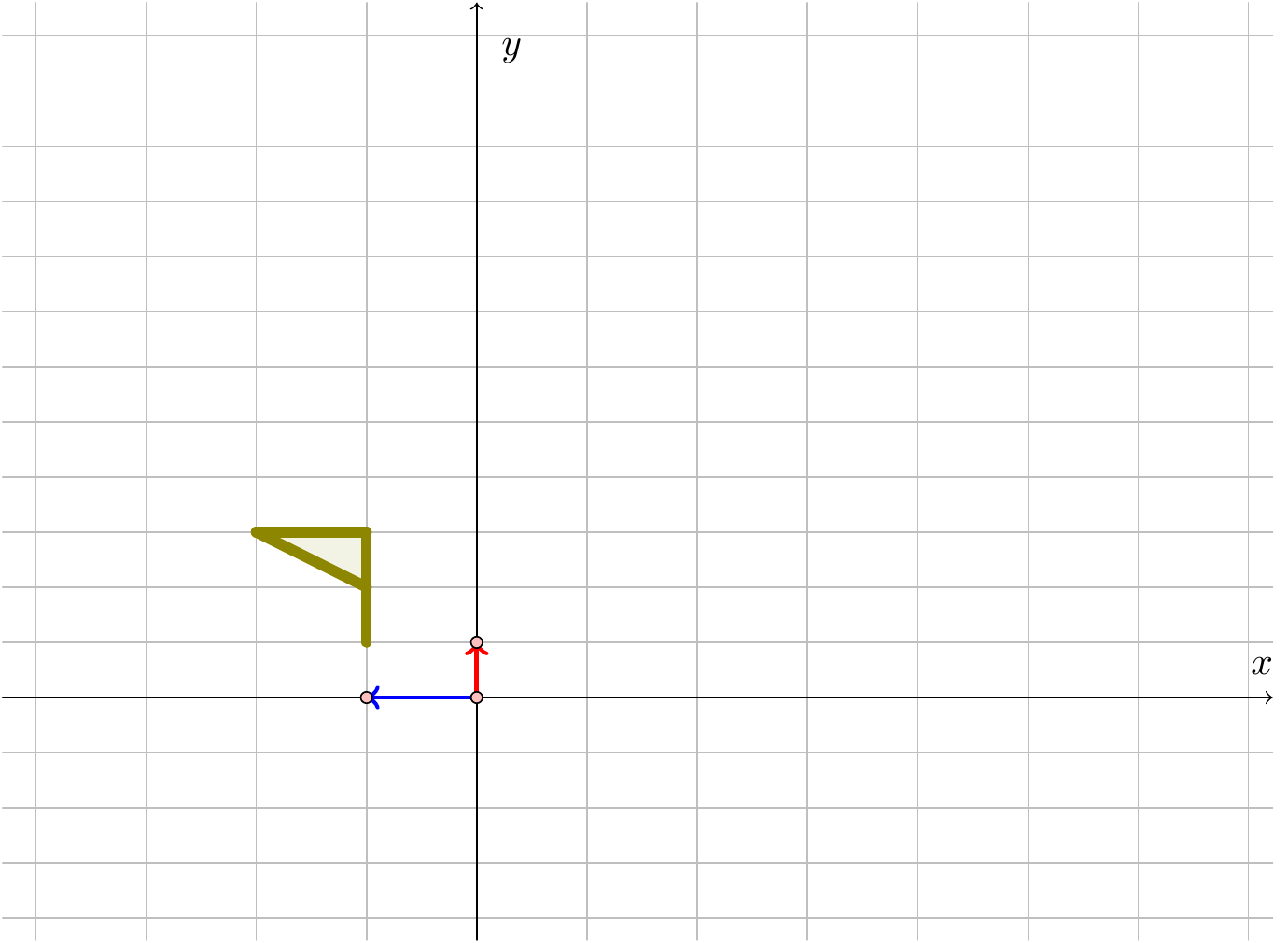
Figure 3.3: The flag after applying \(B\)

So the effect of this matrix is to scale the diagram by a factor of \(-1\) in the \(x\)-direction – i.e., to reflect the graph in the \(y\)-axis – and by a factor of \(\tfrac{1}{2}\) in the \(y\)-direction.

Example 3.3 Consider the matrix \(C=\begin{pmatrix}1&1\\0&1\end{pmatrix}\). Then \(C\begin{pmatrix}x\\y\end{pmatrix}=\begin{pmatrix}x+y\\y\end{pmatrix}\), so \[\begin{aligned} &&C\begin{pmatrix}1\\0\end{pmatrix}=\begin{pmatrix}1\\0\end{pmatrix},\quad C\begin{pmatrix}0\\1\end{pmatrix}=\begin{pmatrix}1\\1\end{pmatrix},\quad C\begin{pmatrix}1\\1\end{pmatrix}=\begin{pmatrix}2\\1\end{pmatrix},\\ &&C\begin{pmatrix}1\\2\end{pmatrix}=\begin{pmatrix}3\\2\end{pmatrix},\quad C\begin{pmatrix}1\\3\end{pmatrix}=\begin{pmatrix}4\\3\end{pmatrix},\quad C\begin{pmatrix}2\\3\end{pmatrix}=\begin{pmatrix}5\\3\end{pmatrix},\end{aligned}\] and we conclude that the diagram above is taken to:

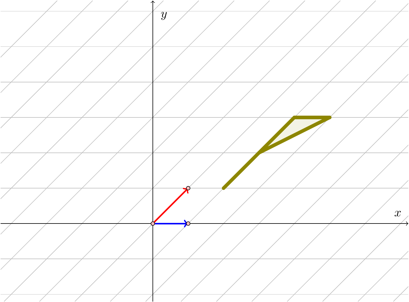
Figure 3.4: The flag after applying \(C\)

This sort of transformation is known as a shear.

Example 3.4 Consider the matrix \(D=\begin{pmatrix}1&-1\\1&1\end{pmatrix}\). Then \[\begin{aligned} &&D\begin{pmatrix}1\\0\end{pmatrix}=\begin{pmatrix}1\\1\end{pmatrix},\quad D\begin{pmatrix}0\\1\end{pmatrix}=\begin{pmatrix}-1\\1\end{pmatrix},\quad D\begin{pmatrix}1\\1\end{pmatrix}=\begin{pmatrix}0\\2\end{pmatrix},\\ &&D\begin{pmatrix}1\\2\end{pmatrix}=\begin{pmatrix}-1\\3\end{pmatrix},\quad D\begin{pmatrix}1\\3\end{pmatrix}=\begin{pmatrix}-2\\4\end{pmatrix},\quad D\begin{pmatrix}2\\3\end{pmatrix}=\begin{pmatrix}-1\\5\end{pmatrix},\end{aligned}\] and we conclude that the diagram above is taken to:

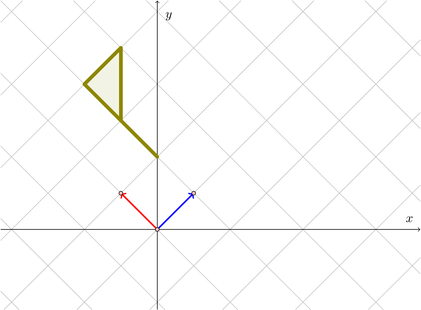
Figure 3.5: The flag after applying \(D\)

This last example looks like a rotation, together with a slight enlargement. We will now consider the general formula for a rotation.

We claim that a rotation by an angle of \(\theta\) gives the following: \[\begin{eqnarray*} X&=&x\cos\theta-y\sin\theta,\\ Y&=&x\sin\theta+y\cos\theta.\end{eqnarray*}\]

Let’s take a point \(P=(x,y)\), and rotate it by an angle of \(\theta\) to get a new point \(P'=(X,Y)\). We claim that the above formulae give \(X\) and \(Y\) in terms of \(x\) and \(y\). Indeed, this follows from the diagram below:

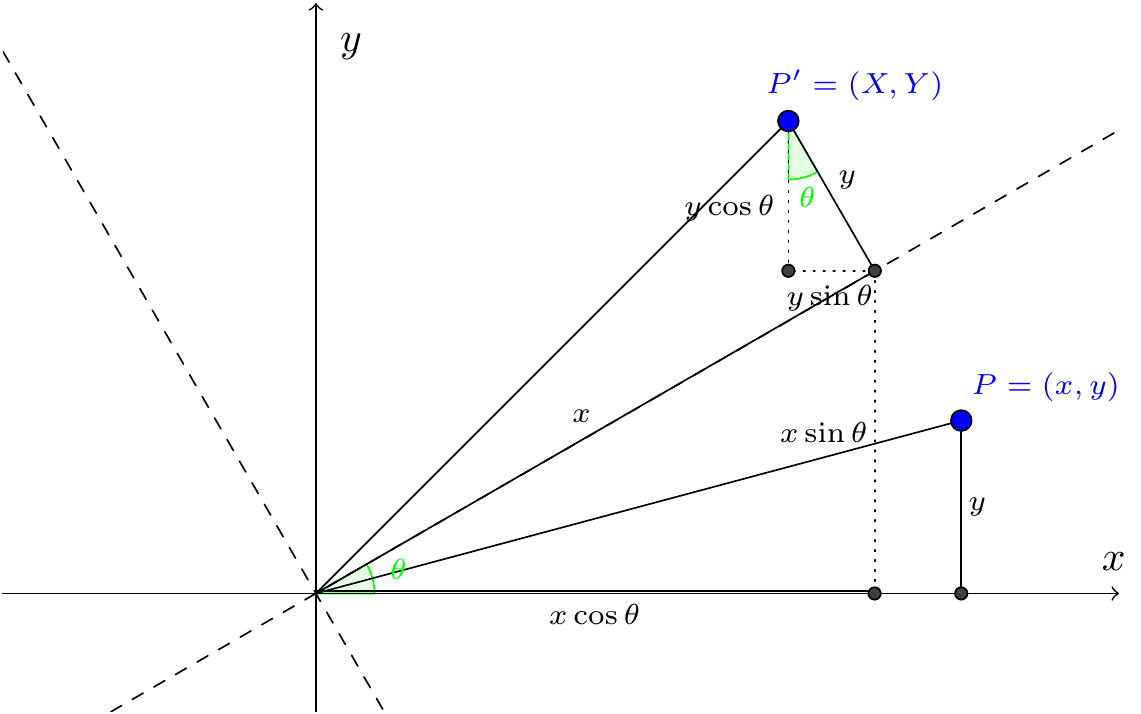
Figure 3.6: Rotation by an angle

This is easily written in matrix form: \[\begin{pmatrix}X\\Y\end{pmatrix}=\begin{pmatrix}\cos\theta&-\sin\theta\\\sin\theta&\cos\theta\end{pmatrix}\begin{pmatrix}x\\y\end{pmatrix}.\] We see that:

The matrix \(\begin{pmatrix}\cos\theta&-\sin\theta\\\sin\theta&\cos\theta\end{pmatrix}\) represents the rotation by \(\theta\).

Now we can see that Example 3.4 is indeed a combination of a rotation and an enlargement; the matrix involved is \[\begin{pmatrix}1&-1\\1&1\end{pmatrix}=\sqrt{2}\begin{pmatrix}1/\sqrt{2}&-1/\sqrt{2}\\1/\sqrt{2}&1/\sqrt{2}\end{pmatrix}=\sqrt{2}\begin{pmatrix}\cos\frac{\pi}{4}&-\sin\frac{\pi}{4}\\\sin\frac{\pi}{4}&\cos\frac{\pi}{4}\end{pmatrix},\] and we now see that the matrix here is a rotation by \(\frac{\pi}{4}\), together with an enlargement by a factor of \(\sqrt{2}\).

Remark. We can view all this in the complex plane. Remember that multiplication by \(e^{i\theta}\) also corresponds to rotating the complex plane by \(\theta\). Suppose that \(z=x+iy\), and so \(e^{i\theta}z=X+iY\) represents the result of rotating by \(\theta\). Since \(e^{i\theta}=\cos\theta+i\sin\theta\), we have \[X+iY=(\cos\theta+i\sin\theta)(x+iy).\] Equating real parts shows that \(X=x\cos\theta-y\sin\theta\), and \(Y=x\sin\theta+y\cos\theta\), as above. (You might like to deduce the formulae for \(\cos(\theta+\phi)\) and \(\sin(\theta+\phi)\) from the fact that a rotation by \(\theta\) followed by a rotation by \(\phi\) is just a rotation by \(\theta+\phi\).)

3.3.3 Matrix multiplication

The definition of the product \(A\mathbf{x}\), and the view of matrix multiplication as a function on vectors, is what gives us the definition of matrix multiplication.

Indeed, given two matrices \(A\) and \(B\), where we suppose that \(A\) is a matrix of size \(m\times p\) and \(B\) is a matrix of size \(q\times n\), we will think of them as functions \(A:\mathbb{R}^p\longrightarrow\mathbb{R}^m\) and \(B:\mathbb{R}^n\longrightarrow\mathbb{R}^q\) respectively. Given two functions, we can try to compose them, that is, do one, and then the other. So we should start with a vector \(\mathbf{x}\) in \(\mathbb{R}^n\), and form \(B\mathbf{x}\), which should be in \(\mathbb{R}^q\). We would like to consider \(A(B\mathbf{x})\), but we can’t do this unless \(p=q\), since we can’t multiply a vector \(B\mathbf{x}\) of length \(q\) by \(A\) if \(p\ne q\), since \(A\) is a function on vectors of length \(p\). So we’ll need \(p=q\) to get this working, and we suppose that this happens. Then we can form \(A(B\mathbf{x})\), a vector of length \(m\), and usual rules of functions mean that this should be \((AB)\mathbf{x}\). We’ll evaluate \(A(B\mathbf{x})\) in a moment, but let’s record the main observation so far:

If \(A\) is an \(m\times p\)-matrix, and \(B\) is a \(q\times n\)-matrix, then we can form the product \(AB\) only if \(p=q\) so the number of columns of \(A\) must equal the number of rows of \(B\)), and then \(AB\) is an \(m\times n\)-matrix.

Suppose \(A\) is an \(m\times p\)-matrix, and that \(B\) is a \(p\times n\)-matrix. We’ll let \(\mathbf{x}\) denote the column vector \(\begin{pmatrix}x_1\\\vdots\\x_n\end{pmatrix}\), a vector of length \(n\).

Given \(\mathbf{x}\), we can work out \(B\mathbf{x}\), and, given our discussion of linear equations, we have: \[B\mathbf{x}=\begin{pmatrix} b_{11}x_1+\cdots+b_{1n}x_n\\ \vdots\\ b_{p1}x_1+\cdots+b_{pn}x_n \end{pmatrix},\] a vector of length \(p\).

In the same way, as \(A\) is an \(m\times p\)-matrix, if \(\mathbf{y}=\begin{pmatrix}y_1\\\vdots\\y_p\end{pmatrix}\), we would want \[A\mathbf{y}=\begin{pmatrix} a_{11}y_1+\cdots+a_{1p}y_p\\ \vdots\\ a_{m1}y_1+\cdots+a_{mp}y_p \end{pmatrix},\] a vector of length \(m\).

Now we work out \(A(B\mathbf{x})\) using the results above, and substituting in \(y_i=b_{i1}x_1+\cdots+b_{in}x_n\): \[A(B\mathbf{x})=\begin{pmatrix} a_{11}(b_{11}x_1+\cdots+b_{1n}x_n)+\cdots+a_{1p}(b_{p1}x_1+\cdots+b_{pn}x_n)\\ \vdots\\ a_{m1}(b_{11}x_1+\cdots+b_{1n}x_n)+\cdots+a_{mp}(b_{p1}x_1+\cdots+b_{pn}x_n) \end{pmatrix}.\] If \(C=(c_{ij})=AB\), then we would want \(C\) to take a vector of length \(n\) to a vector of length \(m\), so \(C\) should be an \(m\times n\)-matrix. Then \(C\mathbf{x}\) should be \[C\mathbf{x}=\begin{pmatrix} c_{11}x_1+\cdots+c_{1n}x_n\\ \vdots\\ c_{m1}x_1+\cdots+c_{mn}x_n \end{pmatrix};\] if we compare the coefficient of \(x_j\) in the \(i\)th entry of \(C\mathbf{x}\) with the same coefficient in \(A(B\mathbf{x})\), we see that \[c_{ij}=a_{i1}b_{1j}+\cdots+a_{ip}b_{pj}=\sum_{k=1}^pa_{ik}b_{kj},\] and this is our definition of matrix multiplication.

So to form the \(ij\)th entry of the product \(C=AB\), we look at the \(i\)th row of \(A\), and the \(j\)th column of \(B\). We have already insisted that these have the same size, so we can form what is essentially the dot product, by adding up the products of the corresponding elements in the \(i\)th row of \(A\) with the elements in the \(j\)th column of \(B\).

For example, if \[A=\begin{pmatrix}1&2\\3&4\end{pmatrix},\quad B=\begin{pmatrix}5&6\\3&9 \end{pmatrix},\] then, if \(C\) denotes the product \(AB\):

• To form \(c_{11}\), we consider \[\begin{aligned} c_{11}&=(\mbox{row 1 of }A)\times(\mbox{column 1 of }B)\\ &=a_{11}b_{11}+a_{12}b_{21}\\ &=1\times5+2\times3=11.\end{aligned}\]

• To form \(c_{12}\), we consider \[\begin{aligned} c_{12}&=(\mbox{row 1 of }A)\times(\mbox{column 2 of }B)\\ &=a_{11}b_{12}+a_{12}b_{22}\\ &=1\times6+2\times9=24.\end{aligned}\]

• In the same way, \[\begin{aligned} c_{21}&=(\mbox{row 2 of }A)\times(\mbox{column 1 of }B)\\ &=a_{21}b_{11}+a_{22}b_{21}\\ &=3\times5+4\times3=27\end{aligned}\] and \[\begin{aligned} c_{22}&=(\mbox{row 2 of }A)\times(\mbox{column 2 of }B)\\ &=a_{21}b_{12}+a_{22}b_{22}\\ &=3\times6+4\times9=54.\end{aligned}\]

Then \[C=\begin{pmatrix} 1&2\\ 3&4 \end{pmatrix}\begin{pmatrix} 5&6\\ 3&9 \end{pmatrix}=\begin{pmatrix} 11&24\\ 27&54 \end{pmatrix}.\]

Similarly, if \[A=\begin{pmatrix} 1&2&3\\ 4&5&6 \end{pmatrix},\quad B=\begin{pmatrix} 2&4\\ -1&-2\\ 5&3 \end{pmatrix},\] then \[C=AB=\begin{pmatrix} 1\times2+2\times(-1)+3\times5&1\times4+2\times(-2)+3\times3\\ 4\times2+5\times(-1)+6\times5&4\times4+5\times(-2)+6\times3 \end{pmatrix}=\begin{pmatrix} 15&9\\ 33&24 \end{pmatrix}.\]

As expected, \(AB\) is a \(2\times 2\)-matrix, since we are taking the product of a \(2\times3\)-matrix with a \(3\times2\)-matrix.

Notice, though, that if we were to multiply them the other way around, and consider \(BA\), we would expect to find a \(3\times3\)-matrix. Convince yourselves of this! And then multiply it out to check!

In most cases \(AB \ne BA\), so matrix multiplication is not commutative.

Example 3.5 If \[A=\begin{pmatrix} 1&2\\ 3&4 \end{pmatrix},\quad B=\begin{pmatrix} 5&6\\ 3&9 \end{pmatrix},\] let’s compute \(AB\) and \(BA\). We’ve already computed \(AB\) above, but we can use the same method to work out \(BA\) and (exercise) the answer is: \[AB=\begin{pmatrix} 11&24\\ 27&54 \end{pmatrix},\qquad BA=\begin{pmatrix} 23&34\\ 30&42 \end{pmatrix}\]

So we see that \(AB\ne BA\).

Example 3.6

If \[A=\begin{pmatrix} 1&2&3\\ 4&5&6 \end{pmatrix},\quad B=\begin{pmatrix} 2&4\\ -1&-2\\ 5&3 \end{pmatrix},\] what are \(AB\) and \(BA\)?

(Indeed, before you do this, what do you expect the sizes of \(AB\) and \(BA\) to be?)

We’ll simply give the answer, so you can check your working. \[AB=\begin{pmatrix} 15&9\\ 33&24 \end{pmatrix},\quad BA=\begin{pmatrix} 18&24&30\\ -9&-12&-15\\ 17&25&33 \end{pmatrix}\]

Not only can \(AB\) and \(BA\) differ, or be of the same size, but one might not even exist. For example, if \(A\) is a \(2\times2\)-matrix, and \(B\) is a \(2\times3\)-matrix, then \(AB\) is a \(2\times3\)-matrix, but we can’t work out \(BA\), since the number of columns of \(B\) is different from the number of rows of \(A\).

You can use the definition of matrix multiplication above to check that for any matrices \(A\), \(B\) and \(C\) of suitable sizes, multiplication is associative, i.e., \[(AB)C=A(BC),\] and we generally simply write \(ABC\) for the answer. But since we defined matrix multiplication as the composition of the corresponding functions, we don’t need to do any of this! We simply just use the fact that composition of functions is always associative, and then we get the result for matrix multiplication.

Similarly, we don’t need to use the formula (although we could!) to see that matrix addition and multiplication are distributive in the sense that \[A(B+C)=AB+AC.\]

3.4 More basic properties

3.4.1 Transpose

Definition 3.2 The transpose operation can be applied to any matrix \(A\) to form its transpose \(A^T\) (also written \(A^t\), or \(A'\)). The rows of \(A^T\) are the columns of \(A\) and the columns of \(A^T\) are the rows of \(A\), taken in the same order.

For example, \[\begin{pmatrix} 1&2\\ 4&6 \end{pmatrix}^T=\begin{pmatrix} 1&4\\ 2&6 \end{pmatrix},\] and \[\begin{pmatrix} 2&7\\ -6&1\\ 0&4 \end{pmatrix}^T=\begin{pmatrix} 2&-6&0\\ 7&1&4 \end{pmatrix}.\] Note that the transpose of an \(m\times n\)-matrix is an \(n\times m\)-matrix.

For any matrix \[\begin{aligned} (A^T)^T&=A,\\ (A+B)^T&=A^T+B^T,\\ (AB)^T&=B^TA^T.\end{aligned}\] The first two of these statements are easy to see. The third is a little trickier. Let’s check it formally.

Proposition 3.1 Suppose that \(A\) is an \(m\times p\)-matrix, and that \(B\) is a \(p\times n\)-matrix. Then \[(AB)^T=B^TA^T.\]

Proof. By definition of the matrix product, the \(ij\)th element of \(AB\) is \[(AB)_{ij}=\sum_{k=1}^na_{ik}b_{kj}.\] Since transposing exchanges the rows and columns, the \(ij\)th element of \((AB)^T\) is the same as the \(ji\)th element of \(AB\), and this is therefore \[(AB)^T_{ij}=\sum_{k=1}^na_{jk}b_{ki},\] the same formula as in the first line, but with \(i\) and \(j\) interchanged.

On the other hand, because \((B^T)_{ik}=b_{ki}\), \((A^T)_{kj}=a_{jk}\), we have \[(B^T A^T)_{ij}=\sum_{k=1}^n(B^T)_{ik}(A^T)_{kj}=\sum_{k=1}^nb_{ki} a_{jk}.\] Now we can see that for any \(i\) and \(j\), the \(ij\)th elements of \((AB)^T\) and \(B^TA^T\) are the same. This gives the result.

Note that the transpose of a row vector is a column vector and vice versa. For example, \[\begin{pmatrix}1&2\end{pmatrix}^T=\begin{pmatrix}1\\2\end{pmatrix},\qquad\begin{pmatrix}3\\4\end{pmatrix}^T=\begin{pmatrix}3&4\end{pmatrix}.\]

Definition 3.3 A square matrix is symmetric if \(A^T=A\). It is antisymmetric or skew-symmetric if \(A^T=-A\).

For example, \[\begin{pmatrix} 1&2\\ 2&3 \end{pmatrix}^T=\begin{pmatrix} 1&2\\ 2&3 \end{pmatrix}\] so it is symmetric. You should see from this example that symmetric matrices have a symmetry about the leading diagonal.

Similarly, \[\begin{pmatrix} 1&2&3\\ 2&3&4\\ 3&4&5 \end{pmatrix}^T=\begin{pmatrix} 1&2&3\\ 2&3&4\\ 3&4&5 \end{pmatrix},\] so this is symmetric too.

An antisymmetric matrix must satisfy \(a_{ij}=-a_{ji}\). In particular, the diagonal elements \(a_{ii}\) must satisfy \(a_{ii}=-a_{ii}\), so \(a_{ii}=0\), and the whole leading diagonal must have zero elements. For the off-diagonal elements, we need \(a_{ij}=-a_{ji}\), so if \[A=\begin{pmatrix} 0&2&1\\ -2&0&3\\ -1&-3&0 \end{pmatrix},\] then \[A^T=\begin{pmatrix} 0&2&1\\ -2&0&3\\ -1&-3&0 \end{pmatrix}^T=\begin{pmatrix} 0&-2&-1\\ 2&0&-3\\ 1&3&0 \end{pmatrix}=-A.\]

For any matrix \(A\), the matrix \(A^TA\) is always symmetric; by the rules we have already seen, \[(A^TA)^T=A^T(A^T)^T=A^TA.\] You might like to check also (or to deduce from this last statement) that \(AA^T\) is also always symmetric.

Example 3.7 If \[A=\begin{pmatrix} 1&2\\ 3&4\\ 5&6 \end{pmatrix},\] then \[A^TA=\begin{pmatrix} 1&3&5\\ 2&4&6 \end{pmatrix}\begin{pmatrix} 1&2\\ 3&4\\ 5&6 \end{pmatrix}=\begin{pmatrix} 35&44\\ 44&56 \end{pmatrix},\] which is clearly symmetric.

3.4.2 The identity matrix \(I\)

In general the \(n\times n\) identity matrix \(I\) is a diagonal matrix where each diagonal element is 1. (Recall that a diagonal matrix is a square matrix where all elements off the leading diagonal are zero.)

So the \(3 \times 3\) identity matrix is \[I=\begin{pmatrix} 1&0&0\\ 0&1&0\\ 0&0&1 \end{pmatrix}.\] You should check that \(I\mathbf{x}=\mathbf{x}\) for any vector \(\mathbf{x}\in\mathbb{R}^3\).

The main property of the identity matrix, and the reason for the terminology, is that if \(A\) is any \(n\times n\) matrix and \(I\) is the \(n\times n\) identity matrix, then \[IA=AI=A.\] As an example, consider \[A=\begin{pmatrix} 2&3\\ 1&2 \end{pmatrix}.\] Then \[IA=\begin{pmatrix} 1&0\\ 0&1 \end{pmatrix}\begin{pmatrix} 2&3\\ 1&2 \end{pmatrix}=\begin{pmatrix} 2&3\\ 1&2 \end{pmatrix},\] and similarly for \(AI\). It’s important here that you try to do this yourself, as you will see exactly why this is working!

3.4.3 The inverse matrix

The collection \(M_n(\mathbb{R})\) of \(n\times n\)-matrices are beginning to look a bit like the collection of all real numbers – we can add, subtract and multiply them (although multiplciation is not commutative). Let’s turn our attention to division.

Definition 3.4 If there exists a matrix \(B\) such that \(AB=BA=I\) then \(B\) is called the inverse of \(A\) and we write \(B=A^{-1}.\)

We shall soon see examples of non-zero matrices that do not have inverses.

Definition 3.5 Only square matrices can have inverses. A square matrix that does not have an inverse is called singular and one that does have an inverse is called non-singular or invertible.

Remark. We could define a left inverse as a matrix \(B\) with \(BA=I\) and a right inverse as a matrix \(C\) with \(AC=I\). It turns out that for square matrices \(A\), any left inverse is also a right inverse and vice versa (even though matrix multiplication is not commutative); to see this, think about \(BAC=(BA)C=B(AC)\).

For the moment, we’ll restrict attention to \(2\times2\)-matrices, but will consider some more general examples later.

Example 3.8 If \[A=\begin{pmatrix} 2&1\\ 7&8 \end{pmatrix},\] then we claim that its inverse is \[B=\begin{pmatrix} \tfrac{8}{9}&-\tfrac{1}{9}\\ -\tfrac{7}{9}&\tfrac{2}{9} \end{pmatrix}.\] To verify this, we simply need to work out \(AB\) and \(BA\), and check that both are the identity.

\[BA=\begin{pmatrix} \tfrac{8}{9}&-\tfrac{1}{9}\\ -\tfrac{7}{9}&\tfrac{2}{9} \end{pmatrix}\begin{pmatrix} 2&1\\ 7&8 \end{pmatrix}=\begin{pmatrix} \tfrac{8}{9}\times2-\tfrac{1}{9}\times7&\tfrac{8}{9}\times1-\tfrac{1}{9}\times8\\ -\tfrac{7}{9}\times2+\tfrac{2}{9}\times7&-\tfrac{7}{9}\times1+\tfrac{2}{9}\times8 \end{pmatrix}=\begin{pmatrix} \tfrac{9}{9}&0\\ 0&\tfrac{9}{9} \end{pmatrix}=\begin{pmatrix} 1&0\\ 0&1 \end{pmatrix},\] and a similar calculation gives \(AB=I\). Thus \(B=A^{-1}\).

In fact, if \(A\) is square (as it has to be for it to have an inverse), you only need to check one of \(AB=I\) and \(BA=I\).

The existence (or otherwise) of the inverse of a square matrix \(A\) depends solely on the value of a number called the determinant of \(A\), which is written \(\det A\). We will see much more about the general theory of determinants in the next chapter.

But we can see this already for \(2\times2\)-matrices.

Example 3.9 Suppose that \[A=\begin{pmatrix}a&b\\c&d\end{pmatrix},\quad B=\begin{pmatrix}d&-b\\-c&a\end{pmatrix}.\] Compute \(AB\) and \(BA\).

You should find that \[AB=BA=\begin{pmatrix}ad-bc&0\\0&ad-bc\end{pmatrix}.\]

This means that if \(ad-bc\ne0\), then \(A\) is invertible, with inverse \[A^{-1}=\frac{1}{ad-bc}\begin{pmatrix}d&-b\\-c&a\end{pmatrix}.\] But if \(ad-bc=0\), i.e., if \(ad=bc\), then this doesn’t work. And in fact, if \(ad=bc\), it isn’t too hard to see that one row of \(A\) must be a multiple of the other, and then there cannot be an inverse for \(A\).

The quantity \(ad-bc\) is the determinant of the \(2\times2\)-matrix \(A=\begin{pmatrix}a&b\\c&d\end{pmatrix}\).

It is possible to define a similar quantity \(\det A\) for all square matrices, with the property that a matrix \(A\) is non-singular if and only if \(\det A\ne0\). We will do this in the next chapter.

Remark. Just to emphasise that this quantity is rather important, let’s consider the pair of simultaneous equations: \[\begin{aligned} ax+by&=s\\ cx+dy&=t.\end{aligned}\] We’d solve these by eliminating \(x\), say, which involves multiplying the first equation by \(c\) and the second by \(a\) to get: \[\begin{aligned} acx+bcy&=cs\\ acx+ady&=at.\end{aligned}\] Then we take the first from the second to get \((ad-bc)y=(at-cs)\); so if \(ad-bc=0\), there are no solutions if \(at-cs\ne0\), and if \(at-cs=0\), then we get the equation \(0=0\).

Proposition 3.2 If \(A\) and \(B\) are invertible \(n\times n\) matrices, then \[(AB)^{-1}=B^{-1}A^{-1}.\]

Proof. Consider \[(B^{-1}A^{-1})AB=B^{-1}(A^{-1}A)B=B^{-1}IB=B^{-1}B=I.\]

3.5 Matrices and linear equations

We have already “abbreviated” systems of linear equations by means of matrices, and viewed these as matrix equations \(A\mathbf{x}=\mathbf{b}\), where if we have \(m\) equations in \(n\) unknowns, then \(A\) is an \(m\times n\) matrix, \(\mathbf{x}\) is the vector of \(n\) unknowns, and \(\mathbf{b}\) is the vector of the \(m\) constant terms in the equations.

3.5.1 Solution of \(A\mathbf{x}=\mathbf{b}\) for invertible matrices \(A\)

Given an equation \(A\mathbf{x}=\mathbf{b}\), we simply (pre-)multiply both sides by \(A^{-1}\) to get \[A^{-1}A\mathbf{x}=A^{-1}\mathbf{b}\] and so \[I\mathbf{x}=A^{-1}\mathbf{b},\] since \(A^{-1}A=I\). But the identity matrix multiplied by anything (as long as the product exists) leaves the result unchanged. So \[\mathbf{x}=A^{-1}\mathbf{b}.\] This means that we have a unique solution of our equations as long as \(A\) is invertible (or, recalling our discussion earlier, if \(\det A\ne0\)).

For \(2\times 2\) system we can use our formula for \(A^{-1}\).

Example 3.10 Consider \[\begin{eqnarray*} 7x+4y&=&15\\ 5x+3y&=&11\end{eqnarray*}\] or given in matrix form \[\begin{pmatrix} 7&4\\ 5&3 \end{pmatrix}\begin{pmatrix}x\\y\end{pmatrix}=\begin{pmatrix}15\\11\end{pmatrix}.\]

First check that \(A^{-1}\) exists: \[\det A=7\times3-4\times5=1,\] and so \[A^{-1}=\frac{1}{1}\begin{pmatrix} 3&-4\\ -5&7 \end{pmatrix},\] so that \[\mathbf{x}=\frac{1}{1}\begin{pmatrix} 3&-4\\ -5&7 \end{pmatrix}\begin{pmatrix}15\\11\end{pmatrix}=\begin{pmatrix}1\\2\end{pmatrix},\] and so we can read off the solution \(x=1\), \(y=2\).

If the matrix \(A\) is not invertible, then this is because we can combine some rows to be a zero row (so the rows are linearly dependent). The corresponding equation is \(0=?\), and if all such equations have the right-hand side \(0\), there will be infinitely many solutions, and otherwise there will be no solutions.

Example 3.11 \[\begin{eqnarray*} 6x+2y&=&10\\ 9x+3y&=&15\end{eqnarray*}\] \(\det A=6\times3-2\times9=0\) so there are infinitely many solutions or no solutions, as \(A\) is singular. In this case, the equations are multiples of one another, so there is really one equation, and there are infinitely many solutions.

All this discussion should lead you to the conclusion that a square matrix \(A\) is invertible precisely when the rows are linearly independent, and that this happens when the Gaussian elimination doesn’t give a complete row of zeros (and that all these are equivalent to the nonvanishing of the determinant, which we will define more later).

3.5.2 Row operations and elementary matrices

We’ve now seen that not only do matrices allow us to abbreviate systems of linear equations, but that this way of writing equations actually comes from some matrix version of the system of equations.

When we solve systems of equations, we generally use Gaussian elimination, and this means doing row operations: swapping rows, scaling a row, or adding a multiple of one row to another.

Let’s point out that all of these operations actually come from matrix multiplication!

Example 3.12 Consider the augmented matrix \[(A|\mathbf{b})=\left(\begin{array}{rrr|r} 3&-1&5&2\\ 6&4&7&5\\ 2&-3&0&6 \end{array}\right).\] Compute \(E(A|\mathbf{b})\) for each of the following matrices \(E\):

1. Firstly, \[E=\begin{pmatrix} 1&0&0\\0&0&1\\0&1&0 \end{pmatrix}.\]

2. Secondly, \[E=\begin{pmatrix} 1&0&0\\0&2&0\\0&0&1 \end{pmatrix}.\]

3. Finally, \[E=\begin{pmatrix} 1&0&2\\0&1&0\\0&0&1 \end{pmatrix}.\]

Try to describe the effect of the multiplications in each case in terms of operations on the rows of the augmented matrix \((A|\mathbf{b})\).

We’ll leave the multiplications to you, but describe the effects of doing these. In the first case, you should find that the second and third rows/equations are interchanged. In the second case, you should find that the second row/equation is doubled, and in the final case, you should find that you are adding two times the third equation onto the first.

In particular, if you do this exercise, and think about what you are doing, you should be able to convince yourself that each operation on the rows of the augmented matrix (or, if you like, each operation on the system of equations) is got by a matrix multiplication.

Since these are the basic operations on systems of equations, these matrices (and any others which perform analogous operations) are known as elementary matrices. Notice that all these operations are obviously invertible by another elementary matrix – the inverse of swapping two rows is to swap them again; the inverse of doubling a row is halving a row; the inverse of adding a multiple of a row to another row is to subtract the same multiple off again.

3.5.3 Computing the inverse matrix

This suggests a method of computing inverse matrices where they exist. Given a matrix \(A\), we do all the row operations as above, to end up with the identity matrix \(I\) (assuming \(A\) is invertible). Since row operations correspond to multiplying successively by matrices, we get \[E_k\ldots E_1A=I.\] This means that \(A^{-1}\) must be \(E_k\ldots E_1\). So how can we find this inverse? Well, we simply do exactly the same operations to the identity matrix \(I\), to end up with \(E_k\ldots E_1I\), and this must be the inverse.

So here is the algorithm (Gauss-Jordan elimination):

Consider the augmented matrix \((A|I)\), where \(A\) is an \(n\times n\)-matrix and \(I\) is the \(n\times n\)-identity matrix.

We do row operations to reduce this matrix to \((I|B)\), using Gaussian elimination, on the columns of \(A\), scaling each row so that \(1\)s are on the diagonal. Then \(B\) is the inverse of \(A\).

Example 3.13 Suppose that \[A=\begin{pmatrix} 1&1&1\\ 2&1&3\\ 2&0&2 \end{pmatrix}.\] Form \[(A|I)=\left(\begin{array}{ccc|ccc} 1&1&1&1&0&0\\ 2&1&3&0&1&0\\ 2&0&2&0&0&1 \end{array}\right)\] and we reduce the left-hand matrix. First let \(R_{2a}=R_2-2R_1\) and \(R_{3a}=R_3-2R_1\): \[\left(\begin{array}{ccc|ccc} 1&1&1&1&0&0\\ 0&-1&1&-2&1&0\\ 0&-2&0&-2&0&1 \end{array}\right).\] Then scale the second equation so that the first entry is \(1\) (\(R_{2b}=-R_{2a}\)): \[\left(\begin{array}{ccc|ccc} 1&1&1&1&0&0\\ 0&1&-1&2&-1&0\\ 0&-2&0&-2&0&1 \end{array}\right)\] Now make the remaining elements in the second column \(0\) by doing \(R_{1a}=R_1-R_{2b}\) and \(R_{3b}=R_{3a}+2R_{2b}\): \[\left(\begin{array}{ccc|ccc} 1&0&2&-1&1&0\\ 0&1&-1&2&-1&0\\ 0&0&-2&2&-2&1 \end{array}\right)\] Now scale the third row (\(R_{3c}=-R_{3b}/2\)) so that it starts with \(1\): \[\left(\begin{array}{ccc|ccc} 1&0&2&-1&1&0\\ 0&1&-1&2&-1&0\\ 0&0&1&-1&1&-1/2 \end{array}\right)\] Finally, make the remaining elements in the third column \(0\) (by \(R_{1b}=R_{1a}-2R_{3c}\) and \(R_{2c}=R_{2b}+R_{3c}\)): \[\left(\begin{array}{ccc|ccc} 1&0&0&1&-1&1\\ 0&1&0&1&0&-1/2\\ 0&0&1&-1&1&-1/2 \end{array}\right)\] and we have reached the desired stage where the left-hand side is the identity matrix. We then read off that \[A^{-1}=\begin{pmatrix} 1&-1&1\\ 1&0&-1/2\\ -1&1&-1/2 \end{pmatrix}.\] (Check by calculation that \(AA^{-1}=A^{-1}A=I\).)

In general, it is far more efficient to solve \(A\mathbf{x}=\mathbf{b}\) by Gauss-elimination and back substitution than by forming \(A^{-1}\) and then \(A^{-1}\mathbf{b}\), but the Gauss-Jordan method is an amusing way to calculate inverses, suitable for implementation by computer.

Corollary 3.1 Every invertible matrix \(A\) is the product of elementary matrices.

Proof. We simply do row reduction on \(A\) until we get down to the identity matrix. Equivalently, we have found elementary matrices \(E_1,\ldots,E_k\) such that \[E_kE_{k-1}\ldots E_1A=I;\] this implies that \[A=E_1^{-1}\ldots E_k^{-1}.\] We have already remarked that the inverse of an elementary matrix is another elementary matrix, and so this shows that \(A\) is itself a product of elementary matrices.

3.5.4 Column operations

You may be wondering why it is row operations which have occupied all our time so far! Partly, of course, this comes from manipulating systems of simultaneous equations.

But there is also a parallel theory of column operations too. Indeed, as an exercise, we suggest taking \(A=\begin{pmatrix}a&b&c\\d&e&f\\g&h&i\end{pmatrix}\), and calculating \(AE\) for each of the elementary matrices \(E\) in Example 3.12.

Indeed, since row reduction corresponds to premultiplying \(A\) by elementary matrices, and column reduction corresponds to postmultiplying \(A\) by elementary matrices, we see in fact that we can do both – first doing row reduction, and then doing column reduction – you might like to try to convince yourself that you can always end up with a matrix whose entries are all \(0\), except for a copy of some identity matrix in the top left-hand corner.

Writing the row reduction matrices as \(P\), and the column matrices as \(Q\), this shows that for any matrix \(A\), there exist \(P\) and \(Q\) such that \(PAQ=\begin{pmatrix}I&0\\0&0\end{pmatrix}\), where \(I\) and \(0\) represent the identity and zero matrices of various sizes.